DSP Based Motion Tracking System
DSP Based Motion Tracking System. Dani Cherkassky Ronen Globinski Advisor: Mr Slapak Alon. Presentation contents. Introduction. Objective The tracking task Utilization potential Design stages. Implementation. System diagram Data flow diagram Tracking flow chart

DSP Based Motion Tracking System
E N D
Presentation Transcript
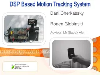
DSP Based Motion Tracking System Dani Cherkassky Ronen Globinski Advisor: Mr Slapak Alon
Presentation contents Introduction • Objective • The tracking task • Utilization potential • Design stages Implementation • System diagram • Data flow diagram • Tracking flow chart • Motion detection algorithm • Tracking algorithm Summery • Conclusions • Future work Results
Introduction Implementation Results Summery Objective Design and implement a DSP based vision system that can detect and track a single, rigid, moving object
Introduction Implementation Results Summery The tracking task • The problem:Detecting and Tracking moving objects in a camera vision field often requires the constant attention of human operators, thus making the tracking task exposed to human errors and working hours problems • The solution: • We offer a DSP based machine vision application that can perform the motion detection and tracking tasks automatically. • Our solution is based on an image processing algorithms that can be implemented on a digital signal processor platform and deliver a real-time performance.
Introduction Implementation Results Summery Utilization potential Motion Detection and tracking system Military systems Traffic control Security Surveillance
Introduction Implementation Results Summery Design stages Stage C Stage A Stage B Stage D Stage E Possible Algorithms Examination (literature survey) Implementing The selected Algorithms (Matlab real time) Implementing The selected Algorithms (DSP platform) Building the Camera motor system Tests and Benchmarks
Implementation Introduction Results Summery System Diagram
Implementation Introduction Results Summery Data Flow Diagram Video Data Flow on the slave DSP board
Implementation Introduction Results Summery Tracking Flow Chart Motion tracking algorithms running on the master DSP board
Implementation Introduction Results Summery Motion Detection Algorithm The principle of the motion detection method is to build a model of the static scene (i.e. without moving objects) called background, and then to compare every frame of the sequence to this background in order to discriminate the regions of unusual motion, called foreground (the moving objects). In this section a motion detection algorithm(∑-∆ filter) proposed by A. Manzanera J. C. Richefeu is introduced. Motion detection , how ??? Methods for motion detection : • Background subtraction algorithms (the naive method) • The background must stay constant • Irrelevant motion is not discarded Not compatible with noisy real world situations! • Last K frames analysis algorithms (histogram , entropy , linear prediction) • Consumes memory (K have to be large) Not suitable for DSP applications ! • Recursive methods that use fixed number of estimates (Kalman filter , ∑-∆ filter) OK! low complexity, low memory consumption, statistical measure on the temporal activity
Implementation Introduction Results Summery Motion Detection Algorithm The ∑-∆ algorithm – a recursive approximation of the temporal statistics, allowing a simple and efficient pixel-level change detection 1 2 Background estimation: Computation of the ∑-∆ mean (an approximation of the median) Motion likelihood measure: Computation of the difference between the image and the median 3 4 Computation of the variance: Defined as the ∑-∆ mean of N times the non-zero differences Motion computation: Comparison between the difference and the variance
Still area Motion area Clutter area Implementation Introduction Results Summery Motion Detection Algorithm Example: two frames from a sequence acquired by a stationary camera Moving object (foreground) Algorithm results for 3 particular pixels from 3 different areas The algorithm can discard irrelevant (clutter) motion - tree moving with the wind, and also has low sensitivity to noise The motion field corresponds to the Boolean indicator of the condition: “the green line is over the black line” – every time the difference is greater than the variance the pixel is considered to be moving.
Implementation Introduction Results Summery Motion Detection Algorithm Example - cont’d The motion field of the moving car The effect of the parameters X, Y, N on the motion field: Salt noise X=1, Y=3, N=4 Filtered X=1, Y=3, N=4 X=1, Y=1, N=4 The sensitivity in this case is too high, thus the motion field is very noisy and unusable Changing the parameter Y affects the variance calculation and in this case lowering the sensitivity which results in a cleaner motion field The motion field can be further cleaned by applying a 3x3 median filter to remove the “salt” noise.
Implementation Introduction Results Summery Motion Tracking Algorithm In this section a method proposed by J. Shi and C. Tomasi is introduced. It is an extension of a method proposed by B. D. Lucas and T. Kanade and will therefore, from now on, be called Extended Lucas-Kanade Tracking (ELKT). Lets look at two sequential frames and express the transformation of the moving object in mathematical terms Image MotionModel (affine motion model) The ELKT is based on the assumption that most changes between two frames are caused by image motion and affine transformations. Affine Model Moving template in Frame 1, Moving template in Frame 2,
Affine transform two samples of the image sequence Implementation Introduction Results Summery Motion Tracking Algorithm We cannot assume perfect correspondence between J(x) and K(Dx + d). This due to image noise and imperfections in the image motion model. There for, some dissimilarity measure should be minimized. In ELKT the sum of squared differences (SSD), is chosen as the dissimilarity measure. Image MotionEstimation This equation would however be non-linear, and therefore difficult to solve. Not a good solution for our DSP Real-time system. Motion estimation = minimizing the dissimilarity . The SSD method ensures that the dissimilarity function has only one minimum. Methods for minimizing the dissimilarity: • The natural approach to minimize the dissimilarity would be • to differentiate the dissimilarity function and set the results to zero. • The better solution is to linearize the function with a truncated Taylor expansion with respect to some good estimate and solve the new system by iterating the procedure.
Implementation Introduction Results Summery Motion Tracking Algorithm The tracking algorithm Tracking = determining the six parameters motion vector µ. The final equation for estimating the six parameters of the Affine motion vector: For each frame n: 1.Calculate µ’(n+1) by iterating this equation. 2.Update the motion vector µ. 3.Use µ to update the position of the target object. The tracking is performed by updating µ using the iterative calculation of µ’ for every input frame. The number of iterations can be determined in advance according to the tracking performance.
It was suggested in [4] to continue the iterations till : • The Advantages of our method are : • No need to measure picture noise level because is an approximation of that level. • Tracking quality is estimated for each frame, it is easy to change the template when that estimate goes low. The average errorcalculated using Alfa filter • Run the EKLT algorithm for a fix number of iterations. • Calculate the tracking error using the next equation : • Check the tracking quality: • If the previous inequality is satisfied continue tracking, else, go back to motion detection. Implementation Introduction Results Summery Motion Tracking Algorithm The EKLT algorithm is recursive, we need to determine the number of iterations • We have found that method problematic for our system because : • T have to be larger then some picture noise level (noise level must be measured). • It may take too long for the algorithm to converge (not capable with RT systems). • We have discovered that if the algorithm doesn't converge after 4-5 iterations there will be practically no convergence at all. Instead of making the exhaustive iterative process we offer a different approach:
Motion detection: O{mxn} , mxn = Frame Size • Feature extraction: O {N} , N = Template Size • Tracking initialization – compute :O {N} • Solving EKLT equation: O {N} Results Introduction Implementation Summery Results • Algorithm Complexity: • CPU Utilization (for 10 x 20 Template size ) : • Motion detection: 82,070,156 (Cycles) • Feature extraction: 20,857 (Cycles) • Tracking initialization: 6,550,668(Cycles) • Solving EKLT equation: 5,205,380(Cycles)
Results Introduction Implementation Summery Results - cont’d • System limitation : The system’s tracking speed is limited • Tracking results : Calculation of the angular velocity of the target object:
Summery Introduction Implementation Results Conclusions • The motion detection algorithm:The ∑-∆ filter, combined with 3x3 median filter, proved to be a robust and accurate method of detection of moving objects for a small cost in memory consumption and computational complexity. • The tracking algorithm:The EKLT tracking algorithm performed well on our system. The algorithm is efficient – the on-line calculations are relatively small and the convergence time is fairly good. The performance can be greatly improved by better selection of the initial features for the tracking process. The good performance of the algorithms proved our concept that a real-time tracking system can be implemented successfully on DSP platforms
Summery Introduction Implementation Results Future work Consider using a DSP with a dual PPI core to improve the performance The DSP implementation must be optimized Improve the pan and tilt mechanism Improve the system’s transition from motion detection to tracking
Summery Introduction Implementation Results References [1] A.Manzanera, J.C.Richefeu "A robust and computationally efficient motion detection algorithm based on Background estimation" [2] G.Jing, C.Eng and D.Rajan. "Foreground motion detection by difference-based spatial temporal entropy" [3] J.Shi and C.Tomashi, "Good Features to Track" Proc. IEEE Conf. Computer Vision and Pattern Recognition, pp.593-600 IEEE CS Press 1994. [4] D.Hager and N.Belhumeur, "Efficient Region Tracking Whit Parametric Models of Geometry and Illumination" IEEE Transaction on Pattern Analysis and Machine Intelligence, Vol. 20, No.10, October 1198.