Acoustic Source Direction by Hemisphere Sampling
120 likes | 146 Vues
This research presents a novel algorithm for determining sound source direction using a compact microphone array setup. Sampled Hemisphere Mapping is utilized to improve accuracy and robustness, eliminating blind spots and following the Principle of Least Commitment. Results show increased performance in real environments. Future work includes integration into a sound source location system and studying multiple simultaneous sound sources.

Acoustic Source Direction by Hemisphere Sampling
E N D
Presentation Transcript
Acoustic Source Direction by Hemisphere Sampling Stanley T. Birchfield Daniel K. Gillmor Quindi Corporation Palo Alto, California
The Problem sound source q f compact microphone array
Previous Work • two microphones f[Huang et al., ICASSP 1999; Stephenne and Champagne, ICASSP 1995] • four microphones q, f[Brandstein et al., ICASSP 1995; Brandstein and Silverman, CSL 1997] • large microphone arrays r, q, f[Brandstein et al., ICASSP 1995; Svaizer et al., ICASSP 1997]
Our microphone array setup microphone d=15cm Note: Arbitrary compact configurations can be handled
Principle of Least Commitment Principle of Least Commitment: “Delay decisions as long as possible” Example:
Previous Algorithm: Cone Intersection decision is made early mic1 signal prefilter find peak correlate mic2 signal prefilter q,f intersect (may be no intersection) mic3 signal prefilter find peak correlate mic4 signal prefilter [Brandstein et al., ICASSP 1995; Brandstein and Silverman, CSL 1997]
Our Algorithm: Sampled Hemisphere map to common coordinate system mic1 signal prefilter correlate sampled hemisphere mic2 signal prefilter correlate final sampled hemisphere … correlate q,f find peak combine correlate correlate temporal smoothing map to common coordinate system mic3 signal prefilter correlate mic4 signal prefilter decision is made after combining all the available evidence
Pair-wise matching of signals microphone mic1 and mic2 mic3 and mic4 all four mics
Sampled Hemisphere asymptotical cones (black regions are theoretical “blind spots”, where cones have no intersection;practical blind spots are larger) sampled hemisphere
Maximum error from matching non-coincident microphones • additional robustness outweighs possible error, which is negligible (less than 5 degrees when r > 4d)
Experimental results(two trials, A and B) A B A B A B Note: also has been extensively used (hundreds of hours) in real environments
Summary • Advantages of sampled hemisphere algorithm • handles arbitrary microphone array configurations • has no “blind spots” • demonstrates increased robustness, by followingthe principle of least commitment • Future work • integrate into a sound source location system • investigate multiple simultaneous sound sources