4.3 NORMAL PROBABILITY DISTRIBUTIONS
420 likes | 573 Vues
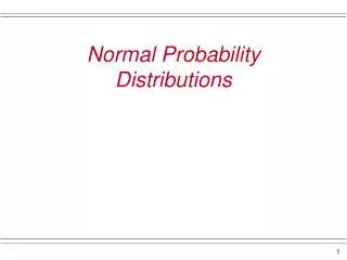
4.3 NORMAL PROBABILITY DISTRIBUTIONS. The Most Important Probability Distribution in Statistics. Normal Distribution . A random variable X with mean m and standard deviation s is normally distributed if its probability density function is given by. Normal Probability Distributions.

4.3 NORMAL PROBABILITY DISTRIBUTIONS
E N D
Presentation Transcript
4.3 NORMAL PROBABILITY DISTRIBUTIONS The Most Important Probability Distribution in Statistics
Normal Distribution • A random variable X with mean m and standard deviation sis normally distributed if its probability density function is given by
Normal Probability Distributions • The expected value (also called the mean) can be any number • The standard deviation can be any nonnegative number • There are infinitely many normal distributions
μ controls location σ controls spread Parameters μ and σ • Normal pdfs have two parameters μ- expected value (mean “mu”)σ- standard deviation (sigma) 7: Normal Probability Distributions
The effects of m and s How does the standard deviation affect the shape of f(x)? s= 2 s =3 s =4 How does the expected value affect the location of f(x)? m = 10 m = 11 m = 12
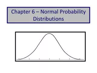
X 0 3 6 9 12 8 µ = 3 and = 1 A family of bell-shaped curves that differ only in their means and standard deviations. µ = the mean of the distribution = the standard deviation
µ = 3 and = 1 X 0 3 6 9 12 µ = 6 and = 1 X 0 3 6 9 12
X 0 3 6 9 12 8 X 0 3 6 9 12 8 µ = 6 and = 2 µ = 6 and = 1
EXAMPLE A Normal Random Variable The following data represent the heights (in inches) of a random sample of 50 two-year old males. (a) Create a relative frequency distribution with the lower class limit of the first class equal to 31.5 and a class width of 1. (b) Draw a histogram of the data. (c ) Do you think that the variable “height of 2-year old males” is normally distributed?
36.0 36.2 34.8 36.0 34.6 38.4 35.4 36.8 34.7 33.4 37.4 38.2 31.5 37.7 36.9 34.0 34.4 35.7 37.9 39.3 34.0 36.9 35.1 37.0 33.2 36.1 35.2 35.6 33.0 36.8 33.5 35.0 35.1 35.2 34.4 36.7 36.0 36.0 35.7 35.7 38.3 33.6 39.8 37.0 37.2 34.8 35.7 38.9 37.2 39.3
68-95-99.7 Rule forNormal Distributions • 68% of the AUC within ±1σ of μ • 95% of the AUC within ±2σ of μ • 99.7% of the AUC within ±3σ of μ 7: Normal Probability Distributions
7: Normal Probability Distributions Wechsler adult intelligence scores: Normally distributed with μ = 100 and σ = 15; X ~ N(100, 15) 68% of scores within μ ± σ= 100 ± 15 = 85 to 115 95% of scores within μ ± 2σ= 100 ± (2)(15) = 70 to 130 99.7% of scores in μ ± 3σ= 100 ± (3)(15) = 55 to 145 Example: 68-95-99.7 Rule
Property and Notation • Property: normal density curves are symmetric around the population mean , so the population mean = population median = population mode = • Notation: X ~ N( is written to denote that the random variable X has a normal distribution with mean and standard deviation .
Standardizing • Suppose X~N( • Form a newrandom variable by subtracting the mean from X and dividing by the standard deviation : (X • This process is called standardizing the random variable X.
Standardizing (cont.) • (X is also a normal random variable; we will denote it by Z: Z = (X • has mean 0 and standard deviation 1:E(Z) = = 0; SD(Z) = = 1. • The probability distribution of Z is called the standard normal distribution.
Standardizing (cont.) • If X has mean and stand. dev. , standardizing a particular value of x tells how many standard deviations x is above or below the mean . • Exam 1: =80, =10; exam 1 score: 92 Exam 2: =80, =8; exam 2 score: 90 Which score is better?
X 0 3 6 9 12 .5 .5 8 (X-6)/2 Z -3 -2 -1 0 1 2 3 µ = 6 and = 2 µ = 0 and = 1
Pdf of a standard normal rv • A normal random variable x has the following pdf:
.5 .5 Z -3 -2 -1 0 1 2 3 Standard Normal Distribution Z = standard normal random variable = 0 and = 1 .5 .5
Important Properties of Z #1. The standard normal curve is symmetric around the mean 0 #2. The total area under the curve is 1; so (from #1) the area to the left of 0 is 1/2, and the area to the right of 0 is 1/2
Finding Normal Percentiles by Hand (cont.) • Table Z is the standard Normal table. We have to convert our data to z-scores before using the table. • The figure shows us how to find the area to the left when we have a z-score of 1.80:
.1587 Z Areas Under the Z Curve: Using the Table P(0 < Z < 1) = .8413 - .5 = .3413 .50 .3413 0 1
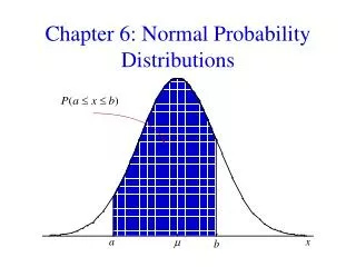
P(- <Z<z0) Standard normal probabilities have been calculated and are provided in table Z. The tabulated probabilities correspond to the area between Z= - and some z0 Z = z0
Example – continued X~N(60, 8) 0.8944 0.8944 0.8944 0.8944 = 0.8944 0.8944 0.8944 P(z < 1.25) In this example z0 = 1.25
Area=.3980 z 0 1.27 Examples • P(0 z 1.27) = .8980-.5=.3980
A2 0 .55 P(Z .55) = A1 = 1 - A2 = 1 - .7088 = .2912
z 0 -2.24 Examples Area=.4875 • P(-2.24 z 0) = Area=.0125 .5 - .0125 = .4875
.1190 Examples (cont.) • P(-1.18 z 2.73) = A - A1 • = .9968 - .1190 • = .8778 .9968 A1 A2 A A1 z -1.18 0 2.73
P(-1 ≤ Z ≤ 1) = .8413 - .1587 =.6826 vi) P(-1≤ Z ≤ 1) .6826 .1587 .8413
6. P(z < k) = .2514 6. P(z < k) = .2514 .5 .5 -.67 .2514 Is k positive or negative? Direction of inequality; magnitude of probability Look up .2514 in body of table; corresponding entry is -.67
Examples (cont.) viii) .7190 .2810
Examples (cont.) ix) .8671 .1230 .9901
.1587 Z P( Z < 2.16) = .9846 .9846 Area=.5 .4846 0 2.16
Example • Regulate blue dye for mixing paint; machine can be set to discharge an average of ml./can of paint. • Amount discharged: N(, .4 ml). If more than 6 ml. discharged into paint can, shade of blue is unacceptable. • Determine the setting so that only 1% of the cans of paint will be unacceptable