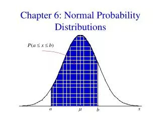
Normal Probability Distributions
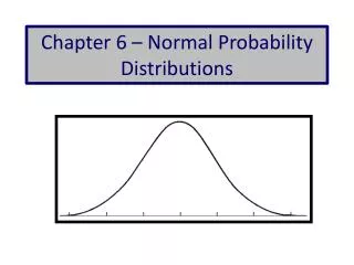
Chapter 5. Normal Probability Distributions. Normal Approximations to Binomial Distributions. § 5.5. Normal Approximation.


Normal Probability Distributions
E N D
Presentation Transcript
Chapter 5 Normal Probability Distributions
Normal Approximations to Binomial Distributions § 5.5
Normal Approximation The normal distribution is used to approximate the binomial distribution when it would be impractical to use the binomial distribution to find a probability. Normal Approximation to a Binomial Distribution If np 5 and nq 5, then the binomial random variable x is approximately normally distributed with mean and standard deviation
Normal Approximation • Example: • Decided whether the normal distribution to approximate x may be used in the following examples. • Thirty-six percent of people in the United States own a dog. You randomly select 25 people in the United States and ask them if they own a dog. • Fourteen percent of people in the United States own a cat. You randomly select 20 people in the United States and ask them if they own a cat. Because np and nq are greater than 5, the normal distribution may be used. Because np is not greater than 5, the normal distribution may NOT be used.
Exact binomial probability P(x = c) Normal approximation P(c 0.5 < x < c + 0.5) c c 0.5 c c + 0.5 Correction for Continuity The binomial distribution is discrete and can be represented by a probability histogram. To calculate exact binomial probabilities, the binomial formula is used for each value of x and the results are added. When using the continuous normal distribution to approximate a binomial distribution, move 0.5 unit to the left and right of the midpoint to include all possible x-values in the interval. This is called the correction for continuity.
Correction for Continuity • Example: • Use a correction for continuity to convert the binomial intervals to a normal distribution interval. • The probability of getting between 125 and 145 successes, inclusive. • The discrete midpoint values are 125, 126, …, 145. • The continuous interval is 124.5 < x < 145.5. • The probability of getting exactly 100 successes. • The discrete midpoint value is 100. • The continuous interval is 99.5 < x < 100.5. • The probability of getting at least 67 successes. • The discrete midpoint values are 67, 68, …. • The continuous interval is x > 66.5.
Guidelines • Using the Normal Distribution to Approximate Binomial Probabilities • In Words In Symbols • Verify that the binomial distribution applies. • Determine if you can use the normal distribution to approximate x, the binomial variable. • Find the mean and standard deviation for the distribution. • Apply the appropriate continuity correction. Shade the corresponding area under the normal curve. • Find the corresponding z-value(s). • Find the probability. Specify n, p, and q. Is np 5? Is nq 5? Add or subtract 0.5 from endpoints. Use the Standard Normal Table.
The variable x is approximately normally distributed with = np = 15.5 and = 15.5 Correction for continuity 13.5 x 10 15 20 Approximating a Binomial Probability Example: Thirty-one percent of the seniors in a certain high school plan to attend college. If 50 students are randomly selected, find the probability that less than 14 students plan to attend college. np = (50)(0.31) = 15.5 nq = (50)(0.69) = 34.5 P(x < 13.5) = P(z < 0.61) = 0.2709 The probability that less than 14 plan to attend college is 0.2079.
= 12 Correction for continuity 10.5 9.5 x 5 10 15 Approximating a Binomial Probability Example: A survey reports that forty-eight percent of US citizens own computers. 45 citizens are randomly selected and asked whether he or she owns a computer. What is the probability that exactly 10 say yes? np = (45)(0.48) = 12 nq = (45)(0.52) = 23.4 = P(0.75 < z 0.45) P(9.5 < x < 10.5) = 0.0997 The probability that exactly 10 US citizens own a computer is 0.0997.