4B: Probability part B Normal Distributions
270 likes | 417 Vues
This lecture provides a comprehensive overview of Normal distributions, which are a key type of continuous random variable in statistics. Covering the history of the Normal function since its recognition by de Moivre and extension by Laplace, this presentation details the probability density function (pdf), the area under the curve (AUC), and characteristics such as the 68-95-99.7 rule. Through illustrative examples, including vocabulary scores and height measurements, we explore how to standardize values using z-scores and find probabilities using the Standard Normal table.

4B: Probability part B Normal Distributions
E N D
Presentation Transcript
4B: Probability part BNormal Distributions 4B: Probability Part B
How’s my hair? Looks good. The Normal distributions • Last lecture covered the most popular type of discrete random variable: binomial variables • This lecture covers the most popular continuous random variable: Normal variables • History of the Normal function • Recognized by de Moivre (1667–1754) • Extended by Laplace (1749–1827) 4B: Probability Part B
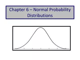
Probability density function (curve) • Illustrative example: vocabulary scores of 947 seventh graders • Smooth curve drawn over histogram is a density function model of the actual distribution • This is the Normal probability density function (pdf) 4B: Probability Part B
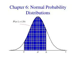
Areas under curve (cont.) • Last week we introduced the idea of the area under the curve (AUC); the same principals applies here • The darker bars in the figure represent scores ≤ 6.0, • About 30% of the scores were less than or equal to 6 • Therefore, selecting a score at random will have probability Pr(X ≤ 6) ≈ 0.30 4B: Probability Part B
Areas under curve (cont.) • Now translate this to a Normal curve • As before, the area under the curve (AUC) = probability • The scale of the Y-axis is adjusted so the total AUC = 1 • The AUC to the left of 6.0 in the figure to the right (shaded) = 0.30 • Therefore, Pr(X ≤ 6) ≈ 0.30 • In practice, the Normal density curve helps us work with Normal probabilities 4B: Probability Part B
Density Curves 4B: Probability Part B
Normal distributions • Normal distributions = a family of distributions with common characteristics • Normal distributions have two parameters • Mean µ locates center of the curve • Standard deviation quantifies spread (at points of inflection) Arrows indicate points of inflection 4B: Probability Part B
68-95-99.7 rule for Normal RVs • 68% of AUC falls within 1 standard deviation of the mean (µ) • 95% fall within 2 (µ2) • 99.7% fall within 3 (µ 3) 4B: Probability Part B
Illustrative example: WAIS Wechsler adult intelligence scores (WAIS) vary according to a Normal distribution with μ = 100 and σ = 15 4B: Probability Part B
Illustrative example: male height • Adult male height is approximately Normal with µ = 70.0 inches and = 2.8 inches (NHANES, 1980) • Shorthand: X ~ N(70, 2.8) • Therefore: • 68% of heights = µ = 70.0 2.8 = 67.2 to 72.8 • 95% of heights = µ 2 = 70.0 2(2.8) = 64.4 to 75.6 • 99.7% of heights = µ 3 = 70.0 3(2.8) = 61.6 to 78.4 4B: Probability Part B
68% (by 68-95-99.7 Rule) ? 16% 16% -1 +1 70 72.8 (height) 84% Illustrative example: male height What proportion of men are less than 72.8 inches tall? (Note: 72.8 is one σ above μ) 4B: Probability Part B
? 68 70 (height) Male Height Example What proportion of men are less than 68 inches tall? 68 does not fall on a ±σ marker. To determine the AUC, we must first standardize the value. 4B: Probability Part B
Standardized value = z score To standardize a value, simply subtract μ and divide by σ This is now a z-score The z-score tells you the number of standard deviations the value falls from μ 4B: Probability Part B
Example: Standardize a male height of 68” Recall X ~ N(70,2.8) Therefore, the value 68 is 0.71 standard deviations below the mean of the distribution 4B: Probability Part B
? 68 70 (height values) Men’s Height (NHANES, 1980) What proportion of men are less than 68 inches tall? = What proportion of a Standard z curve is less than –0.71? -0.71 0 (standardized values) You can now look up the AUC in a Standard Normal “Z” table. 4B: Probability Part B
Using the Standard Normal table Pr(Z≤ −0.71) = .2389 4B: Probability Part B
.2389 68 70 (height values) -0.71 0 (standardized values) Summary (finding Normal probabilities) • Draw curve w/ landmarks • Shade area • Standardize value(s) • Use Z table to find appropriate AUC 4B: Probability Part B
68 70 (height values) -0.71 0 (standardized values) Right tail • What proportion of men are greater than 68” tall? • Greater than look at right “tail” • Area in right tail = 1 – (area in left tail) .2389 1- .2389 = .7611 Therefore, 76.11% of men are greater than 68 inches tall. 4B: Probability Part B
Z percentiles • zp the z score with cumulative probability p • What is the 50th percentile on Z? ANS: z.5 = 0 • What is the 2.5th percentile on Z? ANS: z.025 = 2 • What is the 97.5th percentile on Z? ANS: z.975 = 2 4B: Probability Part B
Finding Z percentile in the table • Look up the closest entry in the table • Find corresponding z score • e.g., What is the 1st percentile on Z? • z.01 = -2.33 • closest cumulative proportion is .0099 4B: Probability Part B
.10 ? 70 (height values) Unstandardizing a value How tall must a man be to place in the lower 10% for men aged 18 to 24? 4B: Probability Part B
Table A:Standard Normal Table • Use Table A • Look up the closest proportion in the table • Find corresponding standardized score • Solve for X (“un-standardize score”) 4B: Probability Part B
Table A:Standard Normal Proportion .08 1.2 .1003 Pr(Z < -1.28) = .1003 4B: Probability Part B
.10 ? 70 (height values) Men’s Height Example (NHANES, 1980) • How tall must a man be to place in the lower 10% for men aged 18 to 24? -1.28 0 (standardized values) 4B: Probability Part B
Observed Value for a Standardized Score • “Unstandardize” z-score to find associated x : 4B: Probability Part B
Observed Value for a Standardized Score • x = μ + zσ = 70 + (-1.28 )(2.8) = 70 + (3.58) = 66.42 • A man would have to be approximately 66.42 inches tall or less to place in the lower 10% of the population 4B: Probability Part B