Normal Probability Distributions
Chapter 5. Normal Probability Distributions. Sampling Distributions and the Central Limit Theorem. § 5.4. Population. Sampling Distributions.


Normal Probability Distributions
E N D
Presentation Transcript
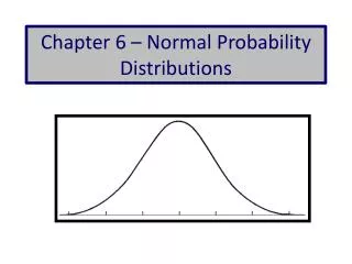
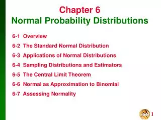
Chapter 5 Normal Probability Distributions
Population Sampling Distributions A sampling distribution is the probability distribution of a sample statistic that is formed when samples of size n are repeatedly taken from a population. Sample Sample Sample Sample Sample Sample Sample Sample Sample Sample
Sample 3 Sample 1 Sample 6 Sample 2 Sample 4 Sample 5 The sampling distribution consists of the values of the sample means, Sampling Distributions If the sample statistic is the sample mean, then the distribution is the sampling distribution of sample means.
Properties of Sampling Distributions • Properties of Sampling Distributions of Sample Means • The mean of the sample means, is equal to the population mean. • The standard deviation of the sample means, is equal to the population standard deviation, divided by the square root of n. • The standard deviation of the sampling distribution of the sample means is called the standard error of themean.
Sampling Distribution of Sample Means • Example: • The population values {5, 10, 15, 20} are written on slips of paper and put in a hat. Two slips are randomly selected, with replacement. • Find the mean, standard deviation, and variance of the population. Population 5 10 15 20 Continued.
Probability Histogram of Population of x P(x) 0.25 Probability x 5 10 15 20 Population values Sampling Distribution of Sample Means • Example continued: • The population values {5, 10, 15, 20} are written on slips of paper and put in a hat. Two slips are randomly selected, with replacement. • Graph the probability histogram for the population values. This uniform distribution shows that all values have the same probability of being selected. Continued.
Sample • Sample mean, • Sample • Sample mean, • 5, 5 • 5 • 15, 5 • 10 • 5, 10 • 7.5 • 15, 10 • 12.5 • 5, 15 • 10 • 15, 15 • 15 • 5, 20 • 12.5 • 15, 20 • 17.5 • 10, 5 • 7.5 • 20, 5 • 12.5 • 10, 10 • 10 • 20, 10 • 15 • 10, 15 • 12.5 • 20, 15 • 17.5 • 10, 20 • 15 • 20, 20 • 20 Sampling Distribution of Sample Means • Example continued: • The population values {5, 10, 15, 20} are written on slips of paper and put in a hat. Two slips are randomly selected, with replacement. • List all the possible samples of size n = 2 and calculate the mean of each. These means form the sampling distribution of the sample means. Continued.
5 • 1 • 0.0625 • 7.5 • 2 • 0.1250 Probability Distribution of Sample Means • 10 • 3 • 0.1875 • 12.5 • 4 • 0.2500 • 15 • 3 • 0.1875 • 17.5 • 2 • 0.1250 • 20 • 1 • 0.0625 Sampling Distribution of Sample Means • Example continued: • The population values {5, 10, 15, 20} are written on slips of paper and put in a hat. Two slips are randomly selected, with replacement. • Create the probability distribution of the sample means.
Probability Histogram of Sampling Distribution P(x) 0.25 0.20 Probability 0.15 0.10 0.05 5 7.5 10 12.5 15 17.5 20 Sample mean Sampling Distribution of Sample Means • Example continued: • The population values {5, 10, 15, 20} are written on slips of paper and put in a hat. Two slips are randomly selected, with replacement. • Graph the probability histogram for the sampling distribution. The shape of the graph is symmetric and bell shaped. It approximates a normal distribution.
The Central Limit Theorem x x x If a sample of size n 30 is taken from a population with any type ofdistributionthat has a mean = and standard deviation = , the sample means will have a normal distribution.
The Central Limit Theorem x x If the population itself is normally distributed, with mean = and standard deviation = , the sample means will have a normal distribution for any sample size n.
The Central Limit Theorem This is also called the standard error of the mean. In either case, the sampling distribution of sample means has a mean equal to the population mean. Mean of the sample means The sampling distribution of sample means has a standard deviation equal to the population standard deviation divided by the square root of n. Standard deviation of the sample means
The Mean and Standard Error Example: The heights of fully grown magnolia bushes have a mean height of 8 feet and a standard deviation of 0.7 feet. 38 bushes are randomly selected from the population, and the mean of each sample is determined. Find the mean and standard error of the mean of the sampling distribution. Standard deviation (standard error) Mean Continued.
Interpreting the Central Limit Theorem Example continued: The heights of fully grown magnolia bushes have a mean height of 8 feet and a standard deviation of 0.7 feet. 38 bushes are randomly selected from the population, and the mean of each sample is determined. The mean of the sampling distribution is 8 feet ,and the standard error of the sampling distribution is 0.11 feet. From the Central Limit Theorem, because the sample size is greater than 30, the sampling distribution can be approximated by the normal distribution.
7.8 Finding Probabilities Example: The heights of fully grown magnolia bushes have a mean height of 8 feet and a standard deviation of 0.7 feet. 38 bushes are randomly selected from the population, and the mean of each sample is determined. The mean of the sampling distribution is 8 feet, and the standard error of the sampling distribution is 0.11 feet. Find the probability that the mean height of the 38 bushes is less than 7.8 feet. Continued.
P( < 7.8) P( < 7.8) = P(z < ____ ) ? 7.8 Finding Probabilities Example continued: Find the probability that the mean height of the 38 bushes is less than 7.8 feet. 1.82 = 0.0344 The probability that the mean height of the 38 bushes is less than 7.8 feet is 0.0344.
P(75 < < 79) z 0 ? ? 75 78 79 Probability and Normal Distributions Example: The average on a statistics test was 78 with a standard deviation of 8. If the test scores are normally distributed, find the probability that the mean score of 25 randomly selected students is between 75 and 79. Continued. 1.88 0.63
P(75 < < 79) z 0 ? ? 75 78 79 Probability and Normal Distributions Example continued: 0.63 1.88 P(75 < < 79) = P(1.88 < z < 0.63) = P(z < 0.63) P(z <1.88) = 0.7357 0.0301 = 0.7056 Approximately 70.56% of the 25 students will have a mean score between 75 and 79.
P( > 35000) 34000 35000 z 0 ? Probabilities of x and x Example: The population mean salary for auto mechanics is = $34,000 with a standard deviation of = $2,500. Find the probability that the mean salary for a randomly selected sample of 50 mechanics is greater than $35,000. = P(z > 2.83) = 1 P(z < 2.83) = 1 0.9977 =0.0023 The probability that the mean salary for a randomly selected sample of 50 mechanics is greater than $35,000 is 0.0023. 2.83
P(x > 35000) 34000 35000 z 0 ? Probabilities of x and x Example: The population mean salary for auto mechanics is = $34,000 with a standard deviation of = $2,500. Find the probability that the salary for one randomly selected mechanic is greater than $35,000. (Notice that the Central Limit Theorem does not apply.) = P(z > 0.4) =1 P(z < 0.4) = 1 0.6554 = 0.3446 The probability that the salary for one mechanic is greater than $35,000 is 0.3446. 0.4
Probabilities of x and x Example: The probability that the salary for one randomly selected mechanic is greater than $35,000 is 0.3446. In a group of 50 mechanics, approximately how many would have a salary greater than $35,000? This also means that 34.46% of mechanics have a salary greater than $35,000. P(x > 35000) = 0.3446 34.46% of 50 = 0.3446 50 = 17.23 You would expect about 17 mechanics out of the group of 50 to have a salary greater than $35,000.