Electromagnetic (E-M) theory of waves at a dielectric interface

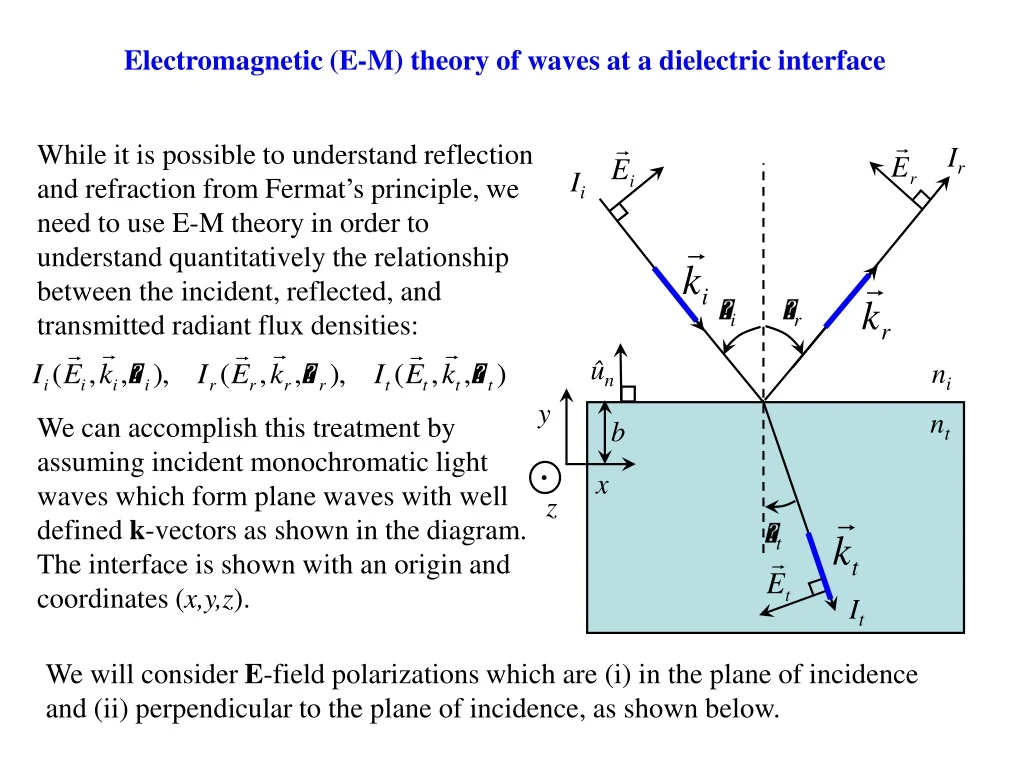
1. i r ûn ni nt b t y . x z Electromagnetic (E-M) theory of waves at a dielectric interface While it is possible to understand reflection and refraction from Fermat’s principle, we need to use E-M theory in order to understand quantitatively the relationship between the incident, reflected, and transmitted radiant flux densities: We can accomplish this treatment by assuming incident monochromatic light waves which form plane waves with well defined k-vectors as shown in the diagram. The interface is shown with an origin and coordinates (x,y,z). Ir Ii It We will consider E-field polarizations which are (i) in the plane of incidence and (ii) perpendicular to the plane of incidence, as shown below.

2. E-field is perpendicular to the plane-of incidence E-field is parallel to the plane of incidence

3. Maxwell’s Equations for time-dependent fields in matter D – Displacement field H – Magnetic Intensity P – Polarization M – Magnetization  - Magnetic permeability  - Permittivity e - Dielectric Susceptibility m - Magnetic Susc. g – Conductivity j – Current density

4. Summary of the boundary conditions for fields at an interface Maxwell’s equations in integral form allow for the derivation of the boundary conditions for the total fields on both sides of a boundary. Side 1 Boundary Side 2 Normal component of D is discontinuous by the free surface charge density Tangential components of E are continuous Normal components of B are continuous Tangential components of H are discontinuous by the free surface current density

5. y . x z For dielectrics, j = 0. Therefore, the components of E and H that are tangent to the interface must be continuous across it. Since we have Ei, Er, and Et the continuity of E components yield:   Note that i r ûn ni nt b t

6. Consider the expression on the interface (y = b) for all x, z and t. The above relationship must hold at all points and at any instant in time on the interface. Therefore Since then we have

7. Thus, at the interface plane  r cos  which is again Snell’s Law

8. Case 1: E  Plane of incidence Continuity of the tangential components of E and H give Cosines cancel Using H = -1B, the tangential components are

9. The last two equations give The symbol  means E  Plane of incidence. These are called the Fresnel equations; most often i t o. Let r = amplitude reflection coefficient and t = amplitude transmission coefficient. Then, the Fresnel equations appear as Note that t - r = 1

10. Case 2: E || Plane of Incidence Continuity of the tangential components of E: Continuity of the tangential components of -1B:

11. If both media forming the interface are non-magnetic i  t  o then the amplitude coefficients become Using Snell’s law the Fresnel Equations for dielectric media become Note that t - r = 1 holds for all i , whereas t|| + r|| = 1 is only true for normal incidence, i.e., i = 0.

12. Consider limiting cases for nearly normal incidence: i  0. In which case, we have: since Also, using the following identity with Snell’s law Therefore, the amplitude reflection coefficient can be written as:

13. In the limiting case for normal incidence i=t= 0, we have : Note that these equalities occur for near normal incidence as a consequence of the fact that the plane of incidence is no longer specified when i  t  0. Consider a specific example of an air-glass interface: i ni = 1 We will consider a particular angle called the Brewster’s angle: p+ t = 90 t nt = 1.5 External reflection nt > ni Internal reflection ni > nt At the polarization angle p, only the component of light polarized normal to the incident plane and therefore parallel to the surface will be reflected.

14. External Reflection (nt > ni) Internal Reflection (nt < ni)

15. Concept of Phase Shifts () in E-M waves: when nt > ni and t < i as in the Air  Glass interface, Since we expect a reversal of sign in the electric field for the Ecase when • We need to define phase shift for two cases: • When two fields E or B are  to the plane of incidence, they are said to be (i) in-phase (=0) if the two E or B fields are parallel and (ii) out-of-phase ( = ) if the fields are anti-parallel. • When two fields E or B are parallel to the plane of incidence, the fields are (i) in-phase if the y-components of the field are parallel and (ii) out-of-phase if the y-components of the field are anti-parallel.

16. Examples of Phase shifts for two particular cases: (a) (b)

17. Analogy between a wave on a string and an E-M wave traversing the air-glass interface. Glass (n = 1.5) Air (n = 1)  = 0  = 0 Air (n = 1) Glass (n = 1.5)  =   = 0 Compare with the case of

18. Examples of phase-shifts using our air-glass interface: In order to understand these phase shifts, it’s important to understand the definition of .

19. Reflected E-field orientations at various angles for the case of External Reflection (ni < nt). It is worth checking and comparing with the various plots for the phase shift  on the previous slides.

20. Reflected E-field orientations at various angles for the case of Internal Reflection (ni > nt). It is worth checking and comparing with the various plots for the phase shift  on the previous slides.

21. Reflectance and Transmittance Remember that the power/area crossing a surface in vacuum (whose normal is parallel to the Poynting vector) is given by The radiant flux density or irradiance (W/m2) is Phase velocity From the geometry and total area A of the beam at the interface, the power (P) for the (i) incident, (ii) reflected and (ii) transmitted beams are:

22. Define Reflectance and Transmittance: Note that Conservation of Energy at the interface yields:

23. Therefore, We can write this expression in the form of componets  and ||: We must use the previously calculated values for

24. It’s possible to verify for the special case of normal incidence: Consider the case of Total Internal Reflection (TIR): t nt = 1 ni = 1.5 i