Decision Trees
Learn about entropy and attribute selection in decision trees. Understand information gain, entropy calculation, and attributes to select for optimal tree construction. Explore examples and gain insights into decision tree building techniques.


Decision Trees
E N D
Presentation Transcript
Decision Trees an introduction
Entropy over the class attribute • A class attribute contains uncertainty over the values • uncertainty captured by entropy H(p) of the target • Increase certainty about the class by considering other attributes • Conditioning (splitting) on an informative attribute produces splits with lower entropy • information gain: entropy before split compared to entropy after split
Yes Age < 35 Rent No Age ≥ 35 Yes Price < 200K Buy No Price ≥ 200K No Other Decision tree • An internal node is a test on an attribute • A branch represents an outcome of the test, e.g., house = Rent • A leaf node represents a class label or class label distribution • At each node, one attribute is chosen to split training examples into distinct classes as much as possible • A new case is classified by following a matching path to a leaf node
Building decision tree, Quinlan 1993 • Top-down tree construction • At start, all training examples are at the root • Partition the examples recursively by choosing one attribute each time. • Bottom-up tree pruning • Remove subtrees or branches, in a bottom-up manner, to improve the estimated accuracy on new cases • Discussed next week
Choosing the splitting attribute • At each node, available attributes are evaluated on the basis of separating the classes of the training examples • A goodness function is used for this purpose • Typical goodness functions: • information gain (ID3/C4.5) • information gain ratio • giniindex (not discussed)
A criterion for attribute selection • Which is the best attribute? • The one which will result in the smallest tree • Heuristic: choose the attribute that produces the purestnodes • Pure and high entropy are opposites • Popular impurity criterion: information gain • Information gain uses entropy H(p) of the class attribute • Information gain increases with the average purity of the subsets that an attribute produces • Strategy: choose attribute that results in greatest information gain
pure, 100% yes not pure at all, 40% yes pure, 100% yes not pure at all, 40% yes Consider entropy H(p) done allmost 1 bit of information required to distinguish yes and no
Entropy Entropy: H(p) = – plg(p) – (1–p)lg(1–p) H(0) = 0 pure node, distribution is skewed H(1) = 0 pure node, distribution is skewed H(0.5) = 1 mixed node, equal distribution
Information gain • Information before split minus information after split • gain(A) = H(p) – ΣH(pi)ni/n • pprobability of positive in current set • nnumber of examples in current set • piprobability of positive in branch i • ninumber of examples in branch i • i before split after split
0lg(0) is not defined, but we evaluate 0lg(0)as zero Example: attribute “Outlook” • Outlook = “Sunny”: H([2,3]) = H(0.4) = −0.4lg(0.4)−0.6lg(0.6) = 0.971 bit • Outlook = “Overcast”: H([4,0]) = H(1) = −1lg(1)−0lg(0) = 0 bit • Outlook = “Rainy”: H([3,2]) = H(0.6) = −0.6lg(0.6)−0.4lg(0.4)= 0.971 bit • Average entropy for Outlook: Weighted sum: (5/14)0.971 + (4/14)0 + (5/14)0.971 = 0.693
Computing the information gain • Information gain for Outlook • gain(Outlook) = H([9,5]) – 0.693 = 0.94 – 0.693 = 0.247 bit • Information gain for attributes from weather data: • gain(Outlook) = 0.247 bit • gain(Temperature) = 0.029 bit • gain(Humidity) = 0.152 bit • gain(Windy) = 0.048 bit
The final decision tree • Note: not all leaves need to be pure; sometimes identical examples have different classes Splitting stops when data can’t be split any further
Highly-branching attributes • Problematic: attributes with a large number of values (extreme case: customer ID) • Subsets are more likely to be pure if there is a large number of values • Information gain is biased towards choosing attributes with a large number of values • This may result in overfitting (selection of an attribute that is non-optimal for prediction)
Split for ID attribute Entropy of each branch = 0 (since each leaf node is pure, having only one case) Information gain is maximal for ID
Gain ratio • Gain ratio: a modification of the information gain that reduces its bias on high-branch attributes • Gain ratio should be • Large when data is divided in few, even groups • Small when each example belongs to a separate branch • Gain ratio takes number and size of branches into account when choosing an attribute • It corrects the information gain by taking the intrinsic information of a split into account (i.e. how much info do we need to tell which branch an instance belongs to)
Gain ratio and intrinsic information • Intrinsic information: entropy of distribution of instances into branches • Gain rationormalizes info gain by:
Computing the gain ratio • Example: intrinsic information for ID • Importance of attribute decreases as intrinsic information gets larger • Example:
More on the gain ratio • Outlook still comes out top • However: ID has greater gain ratio • Standard fix: ad hoc test to prevent splitting on that type of attribute • Problem with gain ratio: it may overcompensate • May choose an attribute just because its intrinsic information is very low • Standard fix: • First, only consider attributes with greater than average information gain • Then, compare them on gain ratio