Download

1 / 38
390 likes | 613 Vues
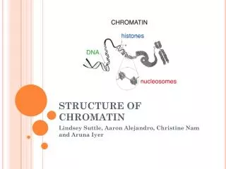
Bioinformatic Analysis of Chromatin Genomic Data. Giulio Pavesi University of Milano giulio.pavesi@unimi.it. Next generation sequencing vs Sanger sequencing http://en.wikipedia.org/wiki/DNA_sequencing. “Nucleosome”.

E N D
Bioinformatic Analysis of Chromatin Genomic Data Giulio Pavesi University of Milano giulio.pavesi@unimi.it
Next generation sequencing vs Sanger sequencing http://en.wikipedia.org/wiki/DNA_sequencing
“Nucleosome” • The nucleosome core particle consists of approximately 147 base pairs of DNA wrapped in 1.67 left-handed superhelical turns around a histone octamer • Octamer: 2 copies each of the core histones H2A, H2B, H3, and H4 • Core particles are connected by stretches of "linker DNA", which can be up to about 80 bp long
Epigenetics • Modern experimental techniques and technologies allow for the genome-wide study of different types of histone modifications, shedding light on the role of each one
The histone code • Example H3K4me3 • H3is the histone • K4 is the residue that is modified and its position (K lysine in position 4 of the sequence) • me3 is the modification (three-methyl groups attached to K4) • If no number at the end like in H3K9ac means only one group
Different chromatin states Chromatin structure (and thus, gene expression) depend also on the post-translational modifications associated with histones forming nuclesomes
“ChIP” • If we have the “right” antibody, we can extract (“immunoprecipitate”) from living cells the protein of interest bound to the DNA • And - we can try to identify which were the DNA regions bound by the protein • Can be done for transcription factors • But can be done also for histones - and separately for each modification
ChIP-Seq Histone ChIP TF ChIP
Many cells- many copies of the same region bound by the protein
After ChIP Size selection: only fragments of the “right size” (200 bp) are kept Identification of the DNA fragment bound by the protein Sequencing
So - if we found that a region has been sequenced many times, then we can suppose that it was bound by the protein, but…
Only a short fragment of the extracted DNA region can be sequenced, at either or both ends (“single” vs “paired end” sequencing) for no more than 35 (before) / 50 (now) / 75 (now) bps Thus, original regions have to be “reconstructed” …and, once again, bioinformaticians can be of help…
Read Mapping • Each sequence read has to be assigned to its original position in the genome • A typical ChIP-Seq experiment produces from 6 (before) to 100 million (now) reads of 50-70 and more base pairs for each sequencing “lane” (Solexa/Illumina) • There exist efficient “sequence mappers” against the genome for NGS read
Read Mapping “Typical” Output @12_10_2007_SequencingRun_3_1_119_647 (actual sequence) TTTGAATATATTGAGAAAATATGACCATTTTT +12_10_2007_SequencingRun_3_1_119_647 (“quality” scores) 40 40 40 40 40 40 40 40 40 40 40 40 40 40 40 40 40 40 40 40 40 40 40 40 40 39 27 40 40 4 27 40
Read Mapping • Reads mapping more than once (repetitive regions) can be discarded: • Never, use all matches everywhere • If they map more than a given maximum number of times • If they do not map uniquely in the best match • If they do not map uniquely with 0, 1, or 2 substitutions
“Peak finding” • The critical part of any ChIP-Seq analysis is the identification of the genomic regions that produced a significantly high number of sequence reads, corresponding to the region where the protein (nucleosome) of interest was bound to DNA • Since a graphical visualization of the “piling” of read mapping on the genome produces a “peak” in correspondence of these regions, the problem is often referred to as “peak finding” • A “peak” then marks the region that was enriched in the original DNA sample
“Peak finding” Peaks: How tall? How wide? How much enriched?
“Peak finding” • The main issue: the DNA sample sequenced (apart from sequencing errors/artifacts) contains a lot of “noise” • Sample “contamination” - the DNA of the PhD student performing the experiment • DNA shearing is not uniform: open chromatin regions tend to be fragmented more easily and thus are more likely to be sequenced • Repetitive sequences might be artificially enriched due to inaccuracies in genome assembly • Amplification pushed too much: you see a single DNA fragment amplified, not enriched • As yet unknown problems, that anyway seem to produce “noisy” sequencings and screw the experiment up
Histone modifications tend to be located at preferred locations with respect to gene annotations/transcribed regions Hence, enrichment can be assessed in two ways Enrichment with respect a the control experiment and peak identification “Local” enrichment in given regions with respect to gene annotations Promoters (active/non active) Upstream of transcribed/non transcribed genes Within transcribed/not transcribed regions Enhancers, whatever else ChIP-Seq histone data
Esperimento • Eseguire una ChIP-Seq per diverse modificazioni istoniche, partendo da quelle più “classiche” • Verificare: • Se ciascuna modifica ha una sua localizzazione “preferenziale” sul genoma o rispetto ai geni (es. nel promotore, nella regione trascritta, etc.) • Se ciascuna modifica è “correlata” in qualche modo alla trascrizione/espressione dei geni
Genome wide histone modifications maps through ChIP-Seq • Barski et.al - Cell 129 823-837, 2007 • 20 histone lysine and arginine methylations in CD4+ T cells • H3K27 • H3K9 • H3K36 • H3K79 • H3R2 • H4K20 • H4R3 • H2BK5 • Plus: • Pol II binding • H2A.Z (replaces H2A in some nucleosomes) • insulator-binding protein (CTCF)
Esperimento • ChIP-Seq associata a una particolare modificazione (es, H3K4me3) • Domanda: la modificazione è “correlabile” alla trascrizione dei geni? • Ovvero, la modificazione “marca” particolari nucleosomi rispetto all’inizio della trascrizione, o alla regione trascritta • Esempio: potrebbero esserci modificazioni che: • Marcano l’inizio della trascrizione • Marcano tutta e solo la regione trascritta • “Silenziano” particolari loci genici impedendo la trascrizione
Esperimento • Sequenze ottenute da ChIP-Seq per la modificazione studiata • Input: coordinate genomiche delle posizioni in ciascuna delle sequenze mappa (vedi file di esempio) • Input: coordinate genomiche dei geni RefSeq annotati • Un nucleosoma marcato dalla modificazione dovrebbe corrispondere a un “mucchietto” di read che si sovrappongono (“picco”) • Andiamo a contare, nucleosoma per nucleosoma, quanto alto è il “mucchietto”, ovvero quanti read sono associabili al nucleosoma
Esempio: se si trovasse la modifica nel nucleosoma a monte del TSS dei geni trascritti, troveremmo un “mucchietto” così Modificazione Nucleosoma
Esempio: se si trovasse la modifica nei nucleosomi associati alle regioni trascritte, troveremmo “mucchietti” così Modificazione Nucleosoma
Analisi: primo esempio • Input • Lista ordinata delle coordinate genomiche dei TSS associati ai geni trascritti • Lista ordinata delle coordinate genomiche dei TSS associati ai geni NON trascritti • Lista ordinata delle coordinate genomiche dove mappa ciascuna sequenza della ChIP-Seq • Output: calcolare la distribuzione (i “mucchietti”) rispetto ai TSS delle due categorie: • Geni trascritti • Geni NON trascritti
Algoritmo! -1000 +1000 TSS Dato ciascun TSS, calcolare quante sequenze mappano tra -1000 e +1000 bp rispetto al TSS Contare quante sequenze mappano a -1000, -999, -998...-1,0 +1,+2,...+998,+999,+1000 Sommare per tutti i TSS i conteggi a ciascuna distanza (-1000, -999, -998,...,-1,0,+1,+2,...+998,+999,+1000)
Attenzione! -1000 +1000 TSS +1000 -1000 TSS Le coordinate rispetto al TSS dipendono dalla direzione della trascrizione!!
Output: histone modifications at TSS Read count (peak height) -1000 0 +1000 Distance from TSS