Parameter, Statistic and Random Samples
Learn about parameters, statistics, sampling, Markov's Inequality, Chebyshev's Inequality, Law of Large Numbers, Central Limit Theorem, and more in probability and statistics.

Parameter, Statistic and Random Samples
E N D
Presentation Transcript
Parameter, Statistic and Random Samples • A parameter is a number that describes the population. It is a fixed number, but in practice we do not know its value. • A statistic is a function of the sample data, i.e., it is a quantity whose value can be calculated from the sample data. It is a random variable with a distribution function. • The random variables X1, X2,…, Xn are said to form a (simple) random sample of size n if the Xi’s are independent random variables and each Xi has the sample probability distribution. We say that the Xi’s are iid. week1
Example • Toss a coin n times. • Suppose • Xi’s are Bernoulli random variables with p = ½ and E(Xi) = ½. • The proportion of heads is . It is a statistic. week1
Sampling Distribution of a Statistic • The sampling distribution of a statistic is the distribution of values taken by the statistic in all possible samples of the same size from the same population. • The distribution function of a statistic is NOT the same as the distribution of the original population that generated the original sample. • Probability rules can be used to obtain the distribution of a statistic provided that it is a “simple” function of the Xi’s and either there are relatively few different values in he population or else the population distribution has a “nice” form. • Alternatively, we can perform a simulation experiment to obtain information about the sampling distribution of a statistic. week1
Markov’s Inequality • If X is a non-negative random variable with E(X) < ∞ and a >0 then, Proof: week1
Chebyshev’s Inequality • For a random variable X with E(X) < ∞ and V(X) < ∞, for any a >0 • Proof: week1
Law of Large Numbers • Interested in sequence of random variables X1, X2, X3,… such that the random variables are independent and identically distributed (i.i.d). Let Suppose E(Xi) = μ , V(Xi) = σ2, then and • Intuitively, as n ∞, so week1
Formally, the Weak Law of Large Numbers (WLLN) states the following: • Suppose X1, X2, X3,…are i.i.d with E(Xi) = μ < ∞ , V(Xi) = σ2 < ∞, then for any positive number a as n ∞ . This is called Convergence in Probability. Proof: week1
Example • Flip a coin 10,000 times. Let • E(Xi) = ½ and V(Xi) = ¼ . • Take a = 0.01, then by Chebyshev’s Inequality • Chebyshev Inequality gives a very weak upper bound. • Chebyshev Inequality works regardless of the distribution of the Xi’s. • The WLLN state that the proportions of heads in the 10,000 tosses converge in probability to 0.5. week1
Strong Law of Large Number • Suppose X1, X2, X3,…are i.i.d with E(Xi) = μ < ∞ , then converges to μ as n ∞ with probability 1. That is • This is called convergence almost surely. week1
Central Limit Theorem • The central limit theorem is concerned with the limiting property of sums of random variables. • If X1, X2,…is a sequence of i.i.d random variables with mean μ and variance σ2 and , then by the WLLN we have that in probability. • The CLT concerned not just with the fact of convergence but how Sn/n fluctuates around μ. • Note that E(Sn) = nμ and V(Sn) = nσ2. The standardized version of Sn is and we have that E(Zn) = 0, V(Zn) = 1. week1
The Central Limit Theorem • Let X1, X2,…be a sequence of i.i.d random variables with E(Xi) = μ < ∞ and Var(Xi) = σ2 < ∞. Let Then, for - ∞ < x < ∞ where Z is a standard normal random variable and Ф(z)is the cdf for the standard normal distribution. • This is equivalent to saying that converges in distribution to Z ~ N(0,1). • Also, i.e. converges in distribution to Z ~ N(0,1). week1
Example • Suppose X1, X2,…are i.i.d random variables and each has the Poisson(3) distribution. So E(Xi) = V(Xi) = 3. • The CLT says that as n ∞. week1
Examples • A very common application of the CLT is the Normal approximation to the Binomial distribution. • Suppose X1, X2,…are i.i.d random variables and each has the Bernoulli(p) distribution. So E(Xi) = p and V(Xi) = p(1- p). • The CLT says that as n ∞. • Let Yn = X1 + … + Xn then Yn has a Binomial(n, p) distribution. So for large n, • Suppose we flip a biased coin 1000 times and the probability of heads on any one toss is 0.6. Find the probability of getting at least 550 heads. • Suppose we toss a coin 100 times and observed 60 heads. Is the coin fair? week1
Sampling from Normal Population • If the original population has a normal distribution, the sample mean is also normally distributed. We don’t need the CLT in this case. • In general, if X1, X2,…, Xn i.i.d N(μ, σ2) then Sn = X1+ X2+…+ Xn ~ N(nμ, nσ2) and week1
Example week1