Modelling and Data Assimilation Techniques for Operational Hydrodynamic Forecast in Tagus Estuary

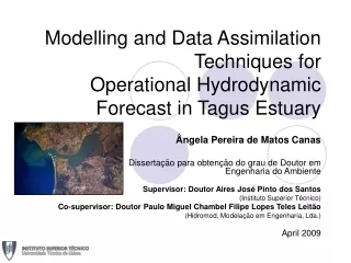
1. Modelling and Data Assimilation Techniques forOperational Hydrodynamic Forecast in Tagus Estuary Ângela Pereira de Matos Canas Dissertação para obtenção do grau de Doutor em Engenharia do Ambiente Supervisor: Doutor Aires José Pinto dos Santos (Instituto Superior Técnico) Co-supervisor: Doutor Paulo Miguel Chambel Filipe Lopes Teles Leitão (Hidromod, Modelação em Engenharia, Lda.) April 2009

2. Contents • Objective • State of the Art • Research Hypotheses • Hypothesis 4 • Conclusions • Future Work

3. Possible to improve hydrodynamic forecast through an alternative model configuration or the use of data assimilation techniques? 1. Objective • Improve the forecast of Tagus Estuary system, contributing to reach operational status.

4. summer Tools to help manage this sensible system? winter • Affecting: • navigation; • biologic production/fishing; • dispersion of domestic/industrial efluents. 2. Tagus Estuary Marshlands Fish/bird nursery Natural Reserve • Largest Portuguese Estuary; • Three distinct parts (Martins, 1999); • Hydrodynamics: • Semi-diurnal tide, max. 2m; • Tagus flow (well mixed estuary); • Wind in coast; • Coastal storms (Gama et al., 1994). Industry Navigation Cities

5. Data assimilation Boundary conditions Integration of scales (processes, grid) Nested modelling (one-way, two-way) Numerical model Validation Data processing Measurement network In-situ (tide gauges, ADCP) Remote sensing River flows Databases Posting Prandle, 2000, Coastal Engineering, 41, 3-12 2. Operational Oceanography • Objective: forecast future conditions; • Components: Operational models Global: HYCOM MERCATOR Regional/local: GoMMOOS PORTS NIVMAR

6. 2. Data Assimilation Tide gauges (SSH,U,V) for Tagus Estuary hydrodynamics

7. assimilation times observations forecast state 2. Sequential Methods • Assimilation in time instants; • Correction of state estimate; • Based on Kalman filter (Kalman, 1960). state ti t0 • Advantages: • - independent of model • support simplifications (adaptation to cost) • possible low complexity • Disadvantages: • - discontinuous state trajectory • required error statistics • assumptions made

8. Data assimilation problem: Extension to non linear models: EKF (Jazwinsky, 1970): linearization of M/H for P and analysis evolution; SEEK (Pham et al., 1998a): [P] = rxr, r << n EnKF (Evensen, 1994): ~ P SEIK (Pham et al., 1998b): ~ P Forecast equation Weakly non linear Observations equation N~100/200 Highly non linear r+1~10 • Kalman filter assumptions: • M, H: linear; • errors: null averaged, gaussian, independent (/); [P] [R] [Q] Suboptimal Optimal nxn nxn pxp [P] = 47963x47963 ! 2. Sequential Methods

9. (Fernandes, 2005) • Several domains: • Barotropic: tide propagation from FES 95.2 solution (Le Provost et al., 1998) – 2D; • Baroclinic: Tagus Estuary – 2D (water quality)/3D (outfall pollution). 24h Forcings: tide, meteo (wind, temperature, heat fluxes, solar radiation, relative humidity) 0.3 Km 2 Km • In-situ: meteorological station, hydrometric station, ocasional ADCP; • Surveys: water/sediment sampling, multiparametric sensor in ship. ? Newtonian relaxation 2. MOHID Tagus Estuary MOHID Water Modelling System (Neves, 1985; Santos, 1995; Martins, 1999; Leitão, 2003) 3D baroclinic primitive equations Validation Posting (http://www.mohid.com/tejo-op/)

10. 3. Research Hypotheses • MOHID Tagus Estuary limitations (Leitão, 2003; Fernandes, 2005): • Model open boundary reference solution: • Tide  Hypothesis 1 • Mean sea level  Hypothesis 2 • Density vertical stratification  Hypothesis 3 • Data assimilation  Hypothesis 4 Not supported Supported Supported

11. 4. Hypothesis 4 - Formulation • Data assimilation of tide gauge measurements with SFEK and SEEK filters: • Improve water level and velocity affected by mean sea level error (2D domain 2); • Evidences: • Estuarine hydrodynamics require very high resolution (Fortunato et al., 1999); • Filters for non linear models at low cost/complexity; • Easily scalable to EnKF or SEIK. 1 – Peniche 6 – Cacilhas 11 - Montijo 2 – Sesimbra 7 – Alfeite 12 - Alcochete 3 – Cascais 8 – Lisboa 13 – Ponta de Erva 4 – Paço de Arcos 9 – Cabo Ruivo 14 – Póvoa de Santa Iria 5 – Trafaria 10 – Seixal 15 – Vila Franca de Xira

12. Implementation in MOHID Water framework: Corrector equations Initialization Analysis error covariance EOF analysis Kalman gain Hydrodynamic_#.hdf5 ... WaterProperties_#.hdf5 Assimilation PreProcessor r << n Analysis Optional correction at initial time Measurements (time series) Filter correction basis L0 Optional reorthonormalization of L Predictor equations State forecast MOHID Water Sequential Assimilation (SFEK, SEEK) Model Modules Forecast error covariance Hydrodynamic WaterProperties Not done in SFEK 4. Hypothesis 4 - Methodology SEEK filter:

13. Assumptions: SEEK: State estimate error described by correction basis L0 in r subspace; Non linear model able to evolve L conserving error representation;  able to represent model errors and filter errors; Traditional: L0 from state estimates variability. 4. Hypothesis 4 - Methodology • Filter parameters: • L0 and dimension of state error subspace r (covariance between all state variables); •  (weighting factor of forecast and observations in analysis, << 1 approach to observations); • R; •  (SEEK).

14. - Tide; • Spatially variable wind (ERA40 reanalysis); • No newtonian relaxation; Tide gauge measurements True model Hypothesis 1 • - Tide; • Spatially variable wind (ERA40 reanalysis); • No newtonian relaxation; • Mean sea level noise N(0, (0.1m)2) Perturbed model Hypothesis 1 4. Hypothesis 4 - Methodology • Application in MOHID Tagus Estuary in Twin Experiment: State = domain 2 (SSH, U, V)

15.  = 0.75 Base filter options: L0from historical model forecasts 4 correction modes 5 measurements every 6 h  = 1 4. Hypothesis 4 - Methodology • Two simulations for 01/10/1972 – 31/01/1973; • EOF analysis of last three months; • Simulations of Perturbed Model with data assimilation (01/11/1972 – 15/11/1972): • SFEK; • SEEK. • Test of several filter options: • ; • composition of L0; • initial correction of state; • measurements: number/frequency.

16. U EOF1 V EOF1 4. Hypothesis 4 - Results SSH EOF1 • EOF analysis: • dominated by tide; • not capturing local hydrodynamics. • 4 EOFs represent 85% of state variability;

17. 5 measurements 10 measurements 4. Hypothesis 4 - Results SFEK • SSH: 5%-25% RMSE reductions; • U, V: not corrected coast and inner estuary, improved with more measurements; • Correction frequency (6h vs 1h) only important in upper estuary. Tagus river ocean SSH analysis: relative RMSE Tagus river ocean U analysis: relative RMSE

18. 5 measurements 10 measurements 4. Hypothesis 4 - Results SEEK • SSH, U, V: corrections inexpressive in most Tagus Estuary; • U, V: degraded in coast. Tagus river ocean SSH analysis relative RMSE Tagus river ocean U analysis relative RMSE

19. Not valid at initial time: • poor corrections especially in velocity fields (coast, estuary); • SFEK correction improved with more locations and frequency of measurements (upper estuary); SFEK correction weak where basis representation is good but where model is known to be highly non linear (Cascais, Sesimbra); 4. Hypothesis 4 - Discussion • Hypothesis not supported! • Assumptions: • Scheme: • State estimate error described by LULT in r space; • Non linear model able to evolve L conserving error representation; • Traditional: • L0 from state estimates variability; • L0 cannot be estimated from whole domain EOF analysis.

20. 5. Conclusions • MOHID Tagus Estuary near state-of-the-art numerical model, requiring improvement in boundary solutions and in data assimilation; • Tide representation mainly limited by bathymetry quality/resolution; • Atmospheric pressure acting on large scale important for water level variability with period above 30h in lower and middle estuary; • Large scale climatological density stratification useful to describe Tagus Estuary mouth stratification; • MOHID Water with simplified Kalman filters easily expandable to more powerful schemes for non linear applications; • Traditional SFEK and SEEK filters unsatisfactory correcting MOHID Tagus Estuary state due to weak representation of state error in correction basis.

21. 6. Future Work • Tide representation: test improved boundary solution (FES 2004) and assess effect of bathymetry; • Assess local effect of wind and atmospheric pressure in mean sea level variability; • Reduce mean sea level bias in MOHID Tagus Estuary; • Test usefulness of large scale model density stratification in improving stratification variability in MOHID Tagus Estuary; • Improve MOHID Water data assimilation module with a learning mechanism for improving filter correction basis (Brasseur et al., 1999) and implement SEIK filter; • Assess data assimilation usefulness in improving water quality.

22. (contract SFRH/BD/14185/2003) (Program INTERREG IIIB – ATLANTIC AREA) (contract SST4-CT-2005-012336) Thank you

24. 3. Hypothesis 1 • Enlargement of domain 1: • Continental Portuguese and Galician Coasts; • Improve tide representation; • Evidences: • Tide error (Leitão, 2003; Fernandes, 2005); • Global tide solution at continental shelf may degrade tide representation (Sauvaget et al., 2000; Leitão, 2003); • Hypothesis not supported.

25. 0.4m ocean Tagus river 4. Hypothesis 2 • Large scale atmospheric pressure effect on mean sea level: • Improve without tide water level representation (2D domain 2); • Evidences: • Storm surge is important in Portuguese Coast (Gama et al., 1994; Ferreira, 2004); • Atmospheric pressure is the dominant cause (Fanjul et al., 1998); • Absent from previous model studies (Leitão, 2003; Fernandes, 2005); • Hypothesis supported.

26. Levitus (1982) climatology 5. Hypothesis 3 • Account thermal and saline vertical stratification: • Improve density stratification (3D domain 2); • Evidences: • Thermal and saline stratification deficiencies (Leitão, 2003; Fernandes, 2005). • Hypothesis supported for outfall area.

27. Analysis evolution with : Hoteit and Pham, 2004, Journal of Marine Systems, 45, 173-188. 6. Hypothesis 4 - Methodology • Assumptions: • Scheme: • State estimate error described by LULT in r space; • Non linear model able to evolve L conserving error representation; •  able to represent model errors and filter errors ( << 1 approach to observations); • SFEK: error variability modes remain fixed in time; • Traditional: • L0 from state estimates variability.

28. assimilation window observations 2. Variational Methods • Assimilation in time interval; • Adjustment of control variables (model parameters, initial/boundary conditions). state ti t0 Advantages: - disperse (space, time) measurements - smooth state trajectory - unrequired state error statistics specification • Disadvantages: • difficult application in operational forecasting • - low flexibility to model changes • - complex development

29. Data assimilation problem: Extension to non linear models: EKF (Jazwinsky, 1970): linearization of M/H for P and analysis evolution; SEEK (Pham et al., 1998a): [P] = rxr, r << n EnKF (Evensen, 1994): ~ P SEIK (Pham et al., 1998b): ~ P Forecast equation Weakly non linear Observations equation N~100/200 Highly non linear EnKF r+1~10 • Kalman filter assumptions: • M, H: linear; • errors: null averaged, gaussian, independent (M/yo); [P] [R] [Q] SEEK SEIK Suboptimal Optimal nxn nxn pxp [P] = 47963x47963 ! 2. Sequential Methods

30. Kalman filter: n = 3: Corrector equations Forecast equation Kalman Gain 3x3 Observations equation Analysis Kalman filter assumptions Analysis error covariance P R Q 3x3 Predictor equations p = 2 (1 and 3): observation operator State forecast 1D schematic case: Forecast error covariance 2x2 2x3 6. Hypothesis 4 - Methodology Data assimilation problem:

31. Implementation in MOHID Water framework: SEEK filter: Corrector equations Initialization Kalman gain EOF analysis Hydrodynamic_#.hdf5 ... WaterProperties_#.hdf5 Assimilation PreProcessor Analysis r << n Analysis error covariance Optional correction at initial time Measurements (time series) Filter correction basis L0 Predictor equations Optional reorthonormalization of L State forecast MOHID Water Sequential Assimilation (SFEK, SEEK) Model Modules Forecast error covariance Hydrodynamic WaterProperties Not done in SFEK 4. Hypothesis 4 - Methodology