Download
1 / 40
400 likes | 484 Vues
09 March 2005 ‘Radar studies on Precipitation, IITM, Pune … madhuchandra r.k. Welcome to Radar Studies on Precipitation MADHU CHANDRA R K, IITM, Pune. Importance & Relevance Background Technological advances.

E N D
09 March 2005 ‘Radar studies on Precipitation, IITM, Pune …madhuchandra r.k Welcome to Radar Studies on Precipitation MADHU CHANDRA R K, IITM, Pune
Importance & Relevance Background Technological advances
Figure 3.3. Height profiles of (a) potential temperature () (circled line) and Relative Humidity (RH) (solid line) (b) vertical wind (w) (circled line) and Richardson number (Ri) (solid line) (c) log (circled line) and log Cn2 (solid line) and (d) wind shear (circled line) and wind speed (Vh)(solid line). All parameters as set (a, b, c and d) associated with particular radiosonde lunch observations correspond to 27 July 1999 at 1630 LT (top panels) and 10 August 1999 at 1800 LT (bottom panels), respectively. The arrow on θ-profile shows the top of the boundary layer. Figure 3.4.HTI sections of diurnal plots of (a) refractive index structure parameter (b) turbulent energy dissipation rate (c) corrected velocity variance (d) wind speed (e) wind shears and (f) vertical wind observed on 27 July 1999. Star marks show the radiosonde estimated boundary layer top.
-8C 5000 -3C 4000 2C Condensation level Altitude (m) 3000 12C 2000 1000 22C Surface 32C
Clouds are visible aggregates of minute water droplets or tiny crystals of ice. Clouds are classified on the basis of their appearance and height. There are three basic cloud types. Cirrus, Stratus, and Cumulus. Cirrus clouds are high, white and thin. The cumulus consists of individual cloud masses with large vertical extent. Stratus clouds are sheets or layers that cover much or all of the sky.
Cloud Droplet Growth Collision-Coalescence
Cloud Drops and Rain Drops Conventional boarder line between cloud drops & rain drops R=100 m V = 70 cm s-1 Typical Condensation Nucleus (CN) R = 0.1 - 1m N = 1000 cm-3 V = 0.001 mm s-1 Typical Cloud Drop R=10 m N = 300 - 500 cm-3 V = 1 cm s-1 Larger Cloud Drop R=50 m N = 10 cm-3 V = 27 cm s-1 Typical Rain Drop R = 1000 m or 1 mm; N= 0.01 cm-3; V = 650 cm s-1
Absorption spectra of atmospheric gases Visible Infrared UV CH4 N2O O2 & O3 CO2 H2O ABSORPTIVITY atmosphere WAVELENGTH (micrometers) IR Windows
Figure 5.3. Average diurnal variation of precipitation from August to November. Figure 5.1. Gadanki four-year rain statistics, like rain accumulation, number of rain events in each year with number of rainy days are presented. Figure 5.2.Monthly rain accumulation information for the years 1998-2001 is shown in panels (a-d) respectively. Gray color columns represent the accumulation contribution from heavy rain. Panel (e) shows the percentage of heavy rain (h.r) contribution to the annual rain accumulation during 1998 to 2001.
MST Radar Antenna Array LAWP ORG Disdrometer Table 2.1. LAWP and MST system and the experimental specifications used for the present study. _____________________________________________________________________ PARAMETER SPECIFICATIONS LAWP MST Radar _____________________________________________________________________ Location Gadanki (13.5N, 79.2E) Antenna (Phased Array) 3.8m X 3.8m 130m X 130m Frequency (f) 1357.5 MHz 53 MHz Radar wave length (lR ) 0.22 m 5.66 m Transmitted peak power (Pt) 1000 Watts 2.5 X 10⁶ Watts Effective aperture (Ae) 10 m2 104 m2 Beam width 43 No. of beams* 3(E15, Zenith & N15) 3(E10, Zenith & N10) Gain (G) 33 dB 36 dB Receiver band width (BN) 1.58 x 10⁶ Hz 1.7 x 10⁶ Hz Receiver path loss (ar) 4 dB 4.4 dB Transmitter path loss (at) 0.5 dB 2.65 dB Cosmic temperature (Tc ) 10 K 6000 K Receiver temperature (Tr) 107 K 607 K Maximum duty ratio 0.05 0.025 Pulse width 1 sec 1 µsec Inter Pulse Period (IPP) 70 msec 1 msec Range resolution (Δr) 150 m 150 m Coherent Integration (NC) 100 128 No. of FFT points 128 128 Observational window: Lowest range bin (km) 0.3 1.5 Highest range bin (km) 9.25 14.25 Incoherent integration 100 1 Beam Dwell time (sec.) 93 17 _____________________________________________________________________ System (s) used
Bright band Figure 2.6b.Representative LAWP observed vertical beam Doppler spectra during convective (top) at 0009 LT, and stratiform (bottom) at 0536 LT on precipitation conditions with their respective moments (a) signal power (b) Doppler shift (c) spectral width and (d) SNR observed on 01 August 1998. Figure 2.6a.Representative clear air time three beams scan, Doppler spectra viz., east (top), north (middle) and zenith/vertical (bottom) with their respective moments (a) signal power (b) Doppler shift (c) spectral width and (d) SNR observed with LAWP on 28 March 2000 at 1009 LT.
Figure 5.7. (a) Isometric plot of LAWP Doppler radar spectra for zenith beam during stratiform rain (b) Isometric plot of LAWP Doppler radar spectra for zenith beam during convective rain. Figure 5.8.Vertical profiles of the range corrected SNR during the presence of bright- band in stratiform rain observed on 01 August 1998.
Received Signal Ranging (Sampling) Coherent integration (Time-Domain Averaging) Spectral analysis (Fast Fourier Transform) Incoherent Integration (Spectral Averaging) Figure 2.5b. Example of a Doppler velocity spectrum observed by the LAWP at 3.45 km at 0227 LT on 02 August 1999. The beam direction is East 15º. Dotted line shows the result of least square fitting to Gaussian function. The gray filled area is the signal power (S) and the hatched area under dashed line is noise power (N). D.C. Removal Spectral Cleaning Noise Level Estimation Spectral moments viz., Echo Power, Doppler Shift and Spectral Width Wind vectors (U, V, & W) Figure 2.5a.Flow chart followed of data processing sequence.
Rayleigh scattering theory can be used to approximate the characteristics of signals reflected back to the radar from precipitation particles (rain, snow, graupel and hail), when the diameter D of the scatterer is small compared to the radar wavelength. The volume reflectivity in this case is given by • = 5 |K|2 Z -4 where Z = NiDi6 is the reflectivity factor in mm6 m-3 and is often expressed by radar meteorologists in the form dBZ equal to 10 log10(Z). The summation is over all drop sizes D, with N, the number of drops in a unit volume. |K|2 is a function of the complex index of refraction of the target equal to 0.93 for liquid water and 0.18 for ice particles. For Rayleigh scattering from spherical particles (i.e., when the diameter D of the particle is small in comparison with the radar wavelength), the backscattering cross-section of a single particle is |K|2 = |(m2-1)/(m2+2)|2
Precipitation studies (Rain Drop Size Distribution) The objectives of this study are…… To see the suitability of two DSD models namely exponential and lognormal model with different combination of moments for observing the characteristic features of tropical rain. To classify stratiform and convective precipitation with the help of LAWP spectra and to study the characteristics of bulk rain integral and lognormal model parameters with respect to stratiform and convective precipitation. To study the natural variation of DSD with respect to mass weighted mean diameter Dm during stratiform and convective precipitation. Tropical precipitation systems using DSD & Doppler spectra
RAIN DROP SIZE DISTRIBUTION (DSD) MODELS Estimation of rain from radars and satellites requires the knowledge of DSD. The DSD is the most versatile rain parameter, by which one can derive many rain integral parameters such as rainfall intensity, liquid water content, radar reflectivity factor, optical extinction, and etc., The exponential and lognormal model parameters can be derived by moment regression method. The moment equation is given by following expression [Ulbrich, 1983], where N(D) is the number density of drops, D is the drop diameter, dD is the increment in drop diameter, Indexed p indicate the respective moment of the drop spectra and ap is a constant for the corresponding pth moment.
The exponential model is expressed by the following equation [Waldvogel, 1974]. N(D)= N0 exp(-D) where N0 = 446.43 W (W/Z) 1.333 and = 6.1196 (W/Z) 0.333 Here N0 (m-3 mm-1) and (mm-1)are the coefficient and slope of DSD curve respectively. To estimate N0 and , liquid water content W (mm3 m-3) and radar reflectivity factor Z (mm6 m-3) are calculated for each observational DSD spectrum of one-minute duration. The model equation for the lognormal distribution is expressed by the following expression [Ajayi and Olsen, 1985] N (D)= (Nt /. (2) .Di) exp [-1/2{(lnDi - ) / } 2] where Nt (m-3) is total number of drops, (mm) is mean of lnD and is standard deviation of the drop spectra which can be expressed as Nt = ao (R) bo ; = A + B ln (R); 2 = A + B ln (R) In the above equation R (mm h-1) is rainfall intensity used as the input parameter, and Di is the drop diameter for ith channel of disdrometer. A, B, A and B are the coefficients of the above equations. These coefficients can be calculated by the moment regression for the combinations of two sets of moments namely (2,3) and (5,6).
Figure 5.6. Comparison of chi square error of observed and model for (a) rainfall rate, for exponential and lognormal distribution (moments 2,3) & moments (5,6) and (b) radar reflectivity factor, for exponential and lognormal distribution for (moments 2,3) & moments (5,6) (c)Comparison of chi square error of ORG observations and model values of rainfall intensity for exponential and lognormal with moments (5,6). Figure 5.5. Comparison of the model DSD with the observed distribution at different rainfall intensity.
Figure 5.9. Scatter plots of (a) M2 Vs R (b) M3 Vs R (c) M4 Vs R (d) M6 Vs R during stratiform rain and (e) M2 Vs R (f) M3 Vs R (g) M4 Vs R (h) M6 Vs R during convective rain.
Figure 5.15.Scatter plot of (a) dBZ Vs Dm (b) R Vs Dm, during stratiform and convective rain. Figure 5.14. Scatter plots of (a) Nt Vs R (b) Vs R and (c)2 Vs R, for Stratiform and Convective rain. During the convective center the value of µ is greater than zero towards positive side. During dissipation stage and stratiform type its value is less than zero. For the same rain rate, in the range of 0.1 to 7.0 mm h -1, the stratiform precipitation has higher value of µ, compared to convective precipitation. However, Nt values for stratiform precipitation system is lower compared to convective precipitation system. During high convective precipitation the values of Dm ≥ 2.0 mm and for stratiform precipitation the average value of Dm ~ 1.5 mm are observed. It is observed that Dm plays an important role in determining the radar reflectivity factor dBZ. Rain fall estimation is very sensitive to the measurements of Dm
Figure 5.12. HTI plot of back scattered signal to noise ratio during convective type of rain on 22-23 June 2000. Figure 5.10. HTI plot of back scattered signal to noise ratio during stratiform rain on 01 August 1998.
Precipitation studies (Rain Drop Size Distribution) The evaporation/precipitation cycle of water has a definite effect on the vertical and horizontal transport of energy in the atmosphere. The spatial and temporal information of precipitation helps in understanding and characterization of the precipitation systems. Potential precipitation parameters like Drop Size Distribution (DSD) can be used to characterize the precipitation. The spatial and temporal distribution of precipitation can be better understood with the availability of height profiles of rain Drop Size Distribution. The purpose of the present work is To retrieve reliable rain DSD height profile using simultaneous observations of UHF and VHF vertically pointing Doppler radar spectra and understanding the height distribution of rain rate and liquid water content with respect to the precipitation systems viz., convective and stratiform. It has observed that lognormal distribution is characterizing Gadanki rain distribution better than exponential distribution. Therefore, the lognormal distribution fit is used for retrieval of DSD from radar Doppler spectra. Estimation of DSD from VHR/UHF Radar Doppler spectra
Z= Rain DSD retrieval: Methodology The backscattered power from the hydrometeors depends upon the size, phase, and number density of the hydrometeors in the pulse volume. The radar reflectivity factor Z due to the hydrometeors varies as the sixth power of the diameter of the hydrometeors summed over all the hydrometeors per unit volume and is expressed as [Doviak and Zrnic ,1993] The lognormal distribution form of N(D) is as follows [Ajayi and Olsen, 1985; Feingold and Levin, 1986] N (D)= (Nt / (2) Di) exp [-1/2{(lnDi - ) / } 2] = (ρ/ρo) 0.45
[a] [b] [c] [f] [d] [e] Figure 6.6.UHF radar zenith beam Doppler spectrums observedduring 2233 LT on 22 June 2000 and 0158 LT on 23 June 2000.
Figure 6.4.Height profile of DSD obtained from representative convective rain Doppler spectra observed during at 2233 LT on 22 June 2000. Height profile extends from 1.8 km to 5.1 km with height resolution 300 m.Each panel consists of observed DSD with and without vertical air velocity corrections shown as bold solid and dotted line respectively. Lognormal least square fit to corrected DSD spectra shown in grey line. Rain rate and Liquid water content estimated from lognormal distribution is given for each height. Figure 6.7.Same as figure 6.4 but it is at 2233 LT on 22 June 2000. Height profile extends from 1.8 km to 5.1 km with height resolution 300 m.
Figure 6.8. Height profile of DSD obtained from representative stratiform rain Doppler spectra observed duringat 0158 LT on 23 June 2000. Height profile extends from 1.5 km to 3.6 km with height resolution 300 m.
Figure 6.9.Estimated height profile of rain rate (R) (black dotted line) and liquid water content (W) (red solid line) from (a and c) convective Doppler spectra and (b and d) stratiform Doppler spectra.
Figure 6.2(a) Rain rates and (b) Liquid water content estimated from radar Doppler spectrums observed at a time interval of every ~10 minutes from 2215 to 0230 LT on 22-23 June 2000.
Gross Conclusions Gadanki rain observational statistics show that the average annual rainfall accumulation is ~ 810 mm. About 66% of annual rain accumulation is due to heavy rain though their occurrence is about 31 %. The rain occurrence rate is more during August to November and it is noticed that their frequency is maximum between 1400 LT and 0600 LT during the day. It is found that lognormal model distribution better characterizes the Gadanki rain in comparison to exponential model. The lognormal model parameter shows good correlation with rainfall rate. This parameter shows positive values for convective rain and negative for stratiform rain. By using the various power law relation between rain rate and DSD moments (rain integral parameters), median volume diameter (Dm) and parameter all together can be used to classify the precipitation systems as convective or stratiform. LAWP vertical beam Doppler spectra shows clear distinguishable features for stratiform and convective precipitation conditions. It is observed that during stratiform precipitation condition, there is strong SNR gradient of order 5 – 15 dB observed at radar bright band level and the Doppler shifts are observed to be around ~ 60 – 70 Hz below the bright band level. During convective precipitation conditions, there is no bright band feature but strong SNR values are found even up to the height of 9 km with Doppler shifts around ~ 60 – 125 Hz. Therefore, these distinct futures of LAWP spectra make feasible to distinguish between convective and stratiform precipitation systems. The LAWP spectral observations enable us to study the height variation of DSD during various precipitation events. The DSD height profile gives an interesting view of vertical structure of precipitation systems. This height profile of DSD also gives an indication of heights where the precipitation is triggered. These studies can thus help in understanding the microphysical properties of clouds. It is observed that the estimated rain rate and liquid water content height profiles, from radar retrieved DSD height profiles, for convective and stratiform rain are different. Moreover, it is possible to determine different stages of the convective precipitation system from the continuous time height profiles of DSD.
Future motivation Challenges 4 u(s)
Challenges 2 U(s) LAWP is unable to probe the first few hundred meter of the atmosphere, i.e. 500 m, from the Earth’s surface. This lower height region which plays a vital role on the structure and dynamics of boundary layer. So, it is important to probe this region using SODAR and tower with fast responding sensors, together with LAWP observations for better understanding the boundary layer structure, turbulent fluxes and convective plumes characteristics. This is particularly important for the studies of nocturnal boundary layer and boundary layer related wave studies such as mountain waves. It is observed that during monsoon season, like LLJ, there exists Tropical Easterly Jet (TEJ) near tropopause height (~ 16 km). The relation between LLJ and TEJ can be studied as a coupled entity to understand the wind systems during monsoon season. The occurrence of occasional peculiar high reflectivity in LAWP observations during nocturnal time, i.e., sunset to sunrise, can be examined in detail to identify the source mechanism associated with such peculiar echoes. During various precipitation events such as SW, NE monsoon systems and convection events Doppler spectra from the LAWP observations can be used to retrieve DSD height profiles. This will help in understanding the cloud microphysical properties associated with various tropical precipitating systems. Simultaneous height profiles of both DSD and meteorological parameters from GPS sonde can be used to estimate the latent heat profiles associated with various tropical precipitation systems. Thank you 4 ur c ooperat ion & pat ience Thank you 4 ur co-operation & patience
Thanks 4 ur c peration & patience ________Ji Hindu
Coming together is a beginning Keeping together is progress Working together is success ________Henry Ford
National MST Radar Facility, Gadanki (13.5oN, 79.2oE)