Production Demonstration Run PDR
Production Demonstration Run PDR. Trainers: Giovanni M. De Santis Bryan C. Book. October 2011. Learning goals. At the end of this training session you will be able to: learn about systems and how they behave; learn about a common approach to improve systems;

Production Demonstration Run PDR
E N D
Presentation Transcript
Production Demonstration RunPDR Trainers: Giovanni M. De Santis Bryan C. Book October 2011
Learning goals • At the end of this training session you will be able to: • learn about systems and how they behave; • learn about a common approach to improve systems; • experience firsthand how to apply an improvement methodology • correctly apply the PDR and related tools to the Supplier’s process
Training agenda Control Practice Information 15’ Welcome and introduction History of Theory of Constraints 15’ Video “The Goal” part 1, lecture and discussion 30’ Video “The Goal” part 2, lecture and discussion 20’ Business Game Run #1 30’ 15’ Discussion 15’ BREAK 20’ Video “The Goal” part 3, lecture and discussion Business Game Run #2 20’ 10’ Discussion Video “The Goal” part 4, lecture and discussion 20’ Buffer Management Lecture 20’ Wrap up and feedback on Theory of Constraints 10’ 60’ LUNCH
Training agenda Control Practice Information 5’ Introduction and scope of PDR procedure 15’ Annexes Exercise annexes 15’ 15’ Feedback and discussion Annexes 20’ Exercise annexes 20’ 15’ Feedback and discussion 15’ BREAK Annexes 40’ 20’ PDR Summery 10’ What to do during PDR 10’ Q&A, final feedback
Basic Class Rules Put cell phones in “vibrate” mode Please close laptops Questions
History of Theory of Constraints • Constraints management started at GM Saginaw Steering Gear in the 1980’s by General Manager Blair Thompson • The physicist Eli Goldratt developed a software program known as Optimized Production Technology (OPT), later writing The Goal. • Eli applied cause-and-effect thinking to manufacturing.
Video: The Goal Part I Jonah gives a cigar out to Alex Duration about 7’ 12”
Discussion: The Goal Part I Alex says ROBOTS increased “Productivity” by 36% !!! Jonah = More $ ??? 1) Sell/Ship more? 2) Costs down? 3) Inventory down? No, actually, not … They are increased… No, quite the opposite…
? Discussion: The Goal Part I • Definition of “Productivity”? • Alex = Improvement in LOCAL Measure ! (the station where the Robots are) • Jonah = Improvement in BOTTOM LINE ! (the yield of the whole plant!) • What was Alex’s Core Problem? • Process used (definition of “system”) and wrong measures/indicators! • What was the Process Alex used? • What did this cause him & his employees to do? • Lose track of the real Goal! • Sub-optimization of the real Goal!
The Improvement Process The “Bottom-Up” Local Improvement Approach
The “TOC” Improvement Process Total System Optimization
Constraints Management Let’s imagine the Organization as a chain of interdependent Activities/Tasks A chain is as strong as its weakest link. It is necessary to work on this link (i.e., constraint) to make the chain stronger.
The Goal – TO MAKE MONEY The main goal for a Company is “to make money now and in the future”. Often, the means to reach the Goal become more important for us than the Goal itself! The means:Customer satisfaction, scrap reduction, cost reduction, etc.
T = Throughput O.E. = Operating Expenses I = Investment Rate at which your money making machine generates new money through sales. New money is sales price less raw materials. Money invested in organization that is ultimately converted into T. Money necessary to convert I onto T. The money making machine I I I I I Money Making Machine Input Output O. E. T T T Crank T T
Throughput Inventory Operating Expenses Constraints Management The Goal: To eliminate or to manage constraints to simultaneously increase throughput and reduce inventory and operating expenses.
Video: The Goal Part II Alex waves goodbye to Jonah after breakfast Duration about 8’ 12”
Discussion: The Goal Part II Op. 10 10 pcs. / h average Op. 20 10 pcs. / h average Op. 30 10 pcs. / h average Op. 40 10 pcs. / h average Op. 50 10 pcs. / h average 9.5 5,9 ? Machine efficiency: 99%. Machine efficiency: 90%. 10 pcs. / h can never be reached. In isolation ðYes In combination ðNo Two crucial elements intervene, which always are detrimental to production: variation and dependence (the higher the variation – average being equal – the larger the difference will be between expected production and real production). Pay attention to how each operation impacts the others and to the system in total. Look for your Bottleneck!!! Constraint !!!
Definition of Weakest link/Constraint “ That element which reduces more strictly the chances of the system to reach the highestperformance with regard to its goals. ”
Kinds of Constraints Capability Offer < Demand Operation A 3000 parts/h Operation B 4000 parts/h Customer’s Demand 5000 parts/h Which is the constraint? Which is the bottleneck? Market Offer > Demand Company Policies Recruitment, overtime, investments, etc.
Business Game: Run #1 • Goal of the business game: to run a simulated factory and discover constraints and bottlenecks • Material available: • card decks • Counters • Card game.xls • Instructions: see notes Practice
? ? ? ? ? Max Buffer = 10 Parts Max Buffer = 10 Parts Max Buffer = 10 Parts Max Buffer = 10 Parts Max Buffer = 10 Parts C C C C Rules of the Game • Cards • Each deck different distribution; • Range: 0 to 10; • Each card represents 1 hour of production; • Shuffle only before Run #1. • Assumptions: • First operation never starved; • Last operation never blocked; • “Pull” (last operation start for first); • Customer’s Demand = 6 parts/h.
Rules of the Game • Run #1 • All buffers limited to 10 maximum; • All buffers initialized at 6 parts each; • Run for 20 hours.
RUN # 1 Where is, in your opinion, the constraint?
Video: The Goal Part III The boy-scouts campfire Duration about 6’18”
Constraints Management Step 0: Define the System. Step 1: Identify the System’s constraint. Step 2: Exploit the System’s constraint. Step 3: Subordinateeverything else to the decisions made in step 2. Step 4: Elevatethe System’s constraint. Step 5: Repeat.If a constraint is broken in step 4, goback to step 1.
Constraints Management Let’s reason with Alex and Jonah treating the “constraint” of the process “walked lane” following the 5 steps we showed: Step 0 -Define: The line of kids + Alex; 1° Step - Identify: Herbie; 2° Step - Exploit: Alex put Herbie at the head of the line; 3° Step - Subordinate: Everybody will walk at Herbie’s pace; Alex unloaded Herbie’s backpack; distributing load; 4° Step - Elevate: 5° Step - Repeat: if anybody will be slower than H., we start again.
Business Game: Run #2 • Goal of the business game: to run a simulated factory and discover how the constraints behave under different conditions • Material available: • card decks • Counters • Card game.xls • Instructions: see notes Practice
Run #2 – differences from Run #1 • All buffers limited to 10 maximum, except for the player immediately before the constraint and the constraint itself (25 max); • All buffers initialized at 6 parts each, except for the player immediately before the constraint (15 parts); • Run for 20 hours.
Video: The Goal Part IV The final scene
Buffers management • Kinds of buffers • We can catalog 3 kinds of buffers: • Parts buffers (A) • Pieces placed before the constraint to avoid its blockage because of lacking feed (“starvation”) • Space buffers (B) • Spaces planned to store parts processed by the constraint to avoid its blockage because the next machine is not processing pieces (“blockage”). • Decoupling buffers (C) • Parts buffers placed between subsystems to separate them from their respective variations.
Buffers management Kinds of buffers C X A B (A) Parts Buffer; (B) Space Buffer; (C) Decoupling Buffer; (X) Constraint.
Buffers management C X A B An insufficient parts buffer causes STARVATION An insufficient space buffer causes BLOCKAGE
Buffers management Correct buffer sizing Parts Buffer before constraint In order to avoid a lack of pieces to be processed by the constraint, it is necessary to measure the longest blockage period of the machine upstream, during a “normal” working period and put into the buffer as many parts as those processed (on average) by that machine during that period. For the constraint machine the entire preceding line is not relevant: just the previous machine should be taken into account.
Buffers management Correct Buffer sizing Space Buffer after constraint In order to avoid a blockage of the constraint, it is necessary to design a space buffer to temporarily place those pieces processed by the constraint which are not machined by the machine downstream (because it is not running). So it is necessary to measure its longest blockage period during a “normal” working period.
Parts Buffer Profile 900 800 700 600 500 Buffer Quantity 400 300 200 Max Min Act 100 0 2-Aug 5-Aug 7-Aug 9-Aug 1-Aug 8-Aug 12-Aug 3-Aug 4-Aug 21-Aug 23-Aug 6-Aug 10-Aug 11-Aug 13-Aug 15-Aug 17-Aug 19-Aug 24-Aug 25-Aug 26-Aug 27-Aug 29-Aug 18-Aug 28-Aug 14-Aug 16-Aug 20-Aug 22-Aug Space Buffer Profile 600 Max Min Act 500 400 Buffer Quantity 300 200 100 - 2-Aug 4-Aug 5-Aug 7-Aug 9-Aug 1-Aug 3-Aug 6-Aug 8-Aug 20-Aug 24-Aug 25-Aug 10-Aug 11-Aug 12-Aug 13-Aug 14-Aug 15-Aug 16-Aug 17-Aug 18-Aug 19-Aug 21-Aug 22-Aug 23-Aug 26-Aug 27-Aug 28-Aug 29-Aug Buffers management Op. 10 Op. 20 Parts Buffer Op. 30 Constraint Operation Space Buffer Op. 40 Op. 50
Key Points • Each system has a constraint • All you have to do is assure a constant parts flow to the constraint • As a team, it is more important to support the constraint operator than anyone else • Buffer management is crucial. It is better to have fewer buffers, but manage them optimally • Buffers must be managed during breaks and overtime • Constraint improvements positively affect the whole system. Improvements of non-constraints are wishful thinking
Key Points • Exploiting the constraint (Step 2), that is, separating it form the variations of the rest of the system by buffers, is very important. If the constraint can produce without being affected by the variations of the system, it will not be faster, but its average throughput will improve (as well as the entire process) and its limits will be optimized. • A mistake to avoid is elevating the constraint (Step 4) immediately after having identified it (Step 1). There is a waste of resources and money (especially with regard to inventory) if non constraints are not subordinated to constraints (Step 3).
Key Points • It doesn’t help if the other operations are faster than the constraint. In fact the manufacturing process begins with raw materials or goods in process which go from the first to the last phase. All operations are important for the process, which cannot be faster than its slowest operation. • Furthermore, subordinating non constraints reduces material storage and circulating capital (cash flow).
Goal of PDR • To verify that the Supplier’s manufacturing process, under normal conditions and according to all customer’s requirements, is able to: • manufacture components / systems / modules that meet all customer requirements; • meet or exceed the production capacity established in the contract / Purchase Order (PO).
What is Daily Tooling Capacity?What do CPG, CPV, and Shift Pattern mean? (Chrysler) • Daily Tooling Capacity (DTC) • It is the supplier’s production capacity of a part, as listed on the PO. • Common Process Group (CPG) • Used when one set of tools produces multiple part numbers. • CPG capacity number is used (instead of adding together the DTC for each part) • Capacity Planning Volume (CPV) • Forecasted volumes based financial planning and options load • Shift Pattern • The operating pattern of the Supplier; in Shifts per day / Hours per Shift / Days per Week (standard is 2/8/5)
Where to find the information (Chrysler) • Log onto the Supplier Quality Portal at https://gsp.extra.chrysler.com/SQP/servlet/SQPServlet • Move mouse to “Summaries” and click on “Part Summary” from the drop-down menu • Enter the part number and click on the “Fetch” box • Click on “Part PO Details” to obtain Tooling Capacity and Operating Pattern
PDR Scope • Applicable to assembly and manufacturing processes for: • Production of new/modified parts; • Carry-over parts with historical quality problems and/or high warranty or which have experienced a Supplier-responsible yard hold within the past calendar year • New and/or additional production lines (e.g. capacity increases) • Production line moves • Any product or process change occurring during the lifecycle of a part or system • Any other component that the SQE determines requires one • Exceptions are allowed only if approved by Quality and Purchasing VP’s of the related Region. (FIAT only)
PDR Leads • Supplier lead at Stage 1 and Stage 2 • Parts identified as “Low” risk in the Initial Risk Evaluation (IRE) • Parts identified as “Supplier-monitored” • Chrysler / FIAT SQE lead at Stage 1, Supplier lead at Stage 2 • Parts identified as “Medium” or “High” risk in the IRE • Parts identified as “Customer-monitored” The SQE may always opt to attend or lead any stage of the PDR, on any part.
PDR Timing (Past & Present) • PDR in 2 stages: • First PDR at Pre Series • 300 pcs or 2 hours minimum • Led by SQE (Medium or High risk; Customer Monitored) • Included in PPAP • Second PDR prior to Job 1 • Data from a full day’s run • Supplier-led (unless SQE decides otherwise) • Not a part of PPAP PDR 300 pcs/ 2 hours Previous 1DP Supplier: full SQE: usually shorter Current PDR #1 300 pcs/ 2 hours SQE PDR #2 Full Day Supplier (SQE)
Responsibility for Capacity • The SQE is responsible for verifying that the Supplier’s production meets the capacity requirements of the contract/PO. • The Buyer is responsible for negotiating with the Supplier in order to assure that the latter is able to support planned volumes.
“How long” and “When?” • Usual duration • Stage 1: 300 pcs or 2 hours, whichever is more stringent • Stage 2: hours per day established in the contract • The SQE can deviate from usual duration with SQ management approval for the following reasons: • - product complexity / usage - conservation and packaging • duration of “production day” - costs • When is it done? • Stage 1: prior to Pre Series (must be completed in time to submit PPAP) • Stage 2: after PPAP, but prior to Job 1 (once Supplier is at or near full production; 4-6 weeks prior is recommended)
Supplier’s preparation • Before the PDR the supplier shall… • perform a PDR test and/or simulations; • For Chrysler Suppliers, the Supplier Readiness Evaluation (SRE) fulfills this requirement • Fill in the PDR work sheets; • Give written confirmation of sub suppliers’ ability to meet Capacity; Quality and Delivery Requirements.