Chapter 2 – Some Important Random Process
Explore the specification, measurement, and important processes of queueing systems alongside the definition and classification of stochastic processes. Learn key concepts and parameters crucial for system analysis.

Chapter 2 – Some Important Random Process
E N D
Presentation Transcript
Chapter 2 – Some Important Random Process Leonard Kleinrock, Queueing Systems, Vol I: Theory Nelson Fonseca, State University of Campinas, Brazil
1.2. Specification and measure of queuing systems • Specification • Distribution of the interarrivals times A(t)=P[time between arrivals ≤t] • Service time distribution B(x)=P[service time ≤ x] • Buffer size • Attendance discipline: • First Come First Served (FCFS) • Last Come First Served (LCFS) • Random • Buffer and service priority
Measurement • Queue size • Waiting time • Idle and busy periods length • Work backlog • Variance and mean
Queueing Systems 2. Some important processes • Cn: The nth customer to enter the system • N(t): Number of customers in the system at time t • U(t): Unfinished work in the system at time x • tn: interarrival time between Cn-1 and Cn = tn - tn-1
If all the interarrivals are drawn from the same distribution, then: P[tn ≤ t]=A(t) • xn: Service time for Cn • Service time drawn from the same distribution P[xn≤x]=B(x)
wn: Waiting time in queue for Cn • sn: Time in system (queue plus service) for Cn sn = wn + xn • Time between arrivals
l – Average arrival rate • Service time
Waiting time Cn • Time in system
sn Cn-1 Cn Cn+1 Cn+2 wn xn xn+1 xn+2 Servicer Cn Cn+1 Cn+2Time tntn+1tn+2 Queue tn+1 tn+2 Cn Cn+1 Cn+2
12 11 10 9 8 7 6 5 4 3 2 1 0 N(t) Number o Customers a(t) d(t)
The total area between curves up to some point t, represents the total time that all customers spent in the system (in units of customer-seconds) during the interval (0,t) – g(t) • l Average customer arrival rate in clients per second during interval (0,x) • Tt Time in system – measurement of all customers in the interval (0,x)
_ • Nt Average number of customers in system during the interval (0,x) • Number of accumulated customers-seconds by total interval length t
Little’s law The average number of users on the queuing system is equal to the average rate of arrivals multiplied by the average time spent in the system • No hypothesis have been made about the arrival time and on the service time • No hypothesis have been made about the limits of the system – it could be queue per server or simply the queue • Nq=lw _
Considering only the server, we have • r utilization factor ratio of the rate at which work enters the system to the maximum rate (capacity) at which the system can handle this work • The work which a user/client brings into the system equals the numbers of seconds of service he requires
r = (average arrival rate of customers) x (average service time) = Single server • Single server Maximum capacity of 1 sec/sec Multiple server • Multiple server capacity of m sec/sec
The rate at which work enters the system is referred to as the traffic intensity of the system and is expressed in Erlangs • In single-server systems, the utilization factor is equal to the traffic intensity • For multiple-server systems, the traffic intensity equals mr r=E[fraction of busy servers]
For the system G/G/1 to be stable, it must be that • For the system D/D/1 r=1 is possible • During the interval t we have: • lt – arrivals • The server is busy during t-tp0 sec • The number of customers served during this interval is • We may now equate the number of arrivals to the number served, which gives:
For the system G/G/1 we have: r – fraction of the time the server is busy • 2.2. Definition and classification of stochastic processes • 3 parameters • State space • Index (time) parameter • Statistical dependencies
State space • Set of possible values that X(t) may take • Discrete-state process countable or finite • State space also referred to as chain • Continuous-state process values in a continuous interval
Distinction between random variables specify joint distribution • Stationary processes • Invariant to shifts in time
Wide sense stationary process First and second moments are independent of t and E[X(t)+X(t+t)]depends only upon t and not upon t Stationary wide sense Stationary wide sense • Independent processes
Markov processes • In a Markov chain the probability that the next value (state) is xn+1 depends only upon the current value and not upon any previous values • The way in which the entire past affects the future of the process is completely summarized in the current value of the process • the state specification cannot contain the information of how long the process has been in that state constraint on the distribution of time (it has to be memoryless) • Continuous case exponential • Discrete case geometrically distributed
P[X(tn+1)=xn+1|X(tn)=xn,X(tn-1)=xn-1,…,X(t1)=x1] =P[X(tn+1)=xn+1|X(tn)=xn] • Birth-death processes • State transition take place between neighboring states only • If Xn=i=>Xn+1=i-1 or Xn+1=i+1
Semi-Markov processes • The discrete–time Markov chain had the property that at every interval the process was required to make a transition from the current state to some other state, possibly back to the same state geometrically distributed • If it is permitted that a process remains an arbitrary time in a state we have a semi-Markov process • At the instants of transition the process behaves just like an ordinary Markov chain embedded Markov chain
Random walks • A particle moving among states the interest is to identify the location of the particle • The next position the process occupies is equal to the previous position plus a random variable whose value is drawn independently from an arbitrary distribution this distribution does not change with time • A sequence of random variables is referred to as a random walk if Sn= X1+ X2+...+ Xn n=1,2,... • Where S0=0 and X1,X2,... is a sequence of independent random variables
n – counts the number of state transitions • If for Xn the distribution is discrete, then we have a discrete-state random walk • pij depends upon the differences of i and j • Renewal processes • Related to a random walk. However, the interest is not in following a particle among many states but rather in counting transitions
The distribution of time between adjacent points is an arbitrary common distribution • The process increases by unity at each transition; X(t) equals the number of state transitions that have taken place by t • q1=1 and qi=0 for i≠1 • Sn=X1+X2+...+Xndenotes the time at which the nth transition takes place
2.3. Discrete-time Markov chains • Example: Hippie who hitchhikes from city to city, travel time is negligible • Definition: the sequence of random variables x1,x2,... forms a discrete-time Markov chain if for all n (x=1,2,...) and all possible values of the random variables we have (for i1<i2<...<in) that P[Xn=j|X1=i1, X2=i2,...,Xn-1=in-1] =P[Xn=j|Xn-1=in-1]
P[Xn=j|X1=i1,X2=i2,...,Xn-1=in-1] one-step transition probability • To determine the state at time n, it is required to know the initial state probability distribution • If the transition probabilities are independent of n, then we have a homogeneous Markov chain:
Homogeneous Markov chains • Transition probabilities are stationary with time – the probability of various states m steps into the future depends only upon m and not upon the current state • From the Markov property we can establish the following recursive formula
To travel from Ei to Ej in m steps, we must do so by first traveling from Ei to some state Ek in m-1 steps and then from Ek to Ej in one step • A Markov chain is irreducible if every state can be reached from every other state; that is, for each pair of states (Ei and Ej) there exists an integer m0 (which may depend upon i and j) such that
A subset of states A1 is said to be closed if no one-step transition is possible from any state in A1 to any state A1c. If A1 consists of a single state then it is called absorbing state. Condition to be an absorbing state is: • If A is not closed and does not contain any proper subset which is closed, then we have an irreducible Markov chain. If A contains proper subsets that are closed, then the chain is said to be reducible
A sub-Markov chain is a irreducible chain which is a subset of a reducible chain can be studied independently • Let • The probability of ever returning to j is given by
Recurrent state fj=1 • Transient fj<1 • Periodic if the only possible steps to return to state Ej are g,2g,3g,…. Periodic with period g • Aperiodic if g=1 • Definition: average time of recurrence • Average time to return to Ej • If Mj=¥ recurrent null • If Mj<¥ recurrent nonnull
Definition: Probability of finding the system in state Ej at the nth step, that is, • Theorem: The states of an irreducible Markov chain are either all transient or all recurrent nonnull or all recurrent null. If periodic, then all states have the same period g.
Definition: stationary distribution {pj} – if we chose it for our initial state distribution (pj(0)=Pj) then for all n we will have pj(n)=Pj Solving for {pj} is a most important part of the analysis of Markov chains • Theorem: In an irreducible and periodic homogeneous Markov chain the limiting probabilities Always exist and are independent of the initial state probability distribution.
Moreover, either (a) all states are transient or all states are recurrent null in which cases pj=0 for all j and there exists no stationary distribution, or (b) all states are recurrent nonnull and then pj>0 for all j, in which case the set {pj} is a stationary probability distribution and
In this case the quantities pj are uniquely determined through the following equations
Definition: A state is said to be ergodic if fi=1, Mj<¥, and g=1. If all states of a Markov chain are ergodic, then the chain itself is ergodic • A Markov chain is said to be ergodic if the probability distribution {pj(n)} as a function of n always converges to a limiting stationary distribution {pj}, which is independent of the initial state distribution • The limiting probabilities {pj}, of an ergodic Markov chain are often referred to as the equilibrium probabilities in the sense that the effect of the initial state distribution pj(0) has disappeared
Probability vector • For the example we have
The solution for p is independent of the initial state vector