7. MOMENT DISTRIBUTION METHOD
7. MOMENT DISTRIBUTION METHOD. 7.1 MOMENT DISTRIBUTION METHOD - AN OVERVIEW. 7.1 MOMENT DISTRIBUTION METHOD - AN OVERVIEW 7.2 INTRODUCTION 7.3 STATEMENT OF BASIC PRINCIPLES 7.4 SOME BASIC DEFINITIONS 7.5 SOLUTION OF PROBLEMS

7. MOMENT DISTRIBUTION METHOD
E N D
Presentation Transcript
7.1 MOMENT DISTRIBUTION METHOD - AN OVERVIEW • 7.1 MOMENT DISTRIBUTION METHOD - AN OVERVIEW • 7.2 INTRODUCTION • 7.3 STATEMENT OF BASIC PRINCIPLES • 7.4 SOME BASIC DEFINITIONS • 7.5 SOLUTION OF PROBLEMS • 7.6 MOMENT DISTRIBUTION METHOD FOR STRUCTURES HAVING NONPRISMATIC MEMBERS
7.2 MOMENT DISTRIBUTION METHOD - INTRODUCTION AND BASIC PRINCIPLES 7.1 Introduction (Method developed by Prof. Hardy Cross in 1932) The method solves for the joint moments in continuous beams and rigid frames by successive approximation. 7.2 Statement of Basic Principles Consider the continuous beam ABCD, subjected to the given loads, as shown in Figure below. Assume that only rotation of joints occur at B, C and D, and that no support displacements occur at B, C and D. Due to the applied loads in spans AB, BC and CD, rotations occur at B, C and D. 150 kN 15 kN/m 10 kN/m 3 m A D B C I I I 8 m 6 m 8 m
In order to solve the problem in a successively approximating manner, it can be visualized to be made up of a continued two-stage problems viz., that of locking and releasing the joints in a continuous sequence. 7.2.1 Step I The joints B, C and D are locked in position before any load is applied on the beam ABCD; then given loads are applied on the beam. Since the joints of beam ABCD are locked in position, beams AB, BC and CD acts as individual and separate fixed beams, subjected to the applied loads; these loads develop fixed end moments. 15 kN/m 10 kN/m -80 kN.m -80 kN.m -112.5kN.m -53.33 kN.m 112.5 kN.m 53.33 kN.m 150 kN 3 m A B C D B 8 m C 8 m 6 m
In beam AB Fixed end moment at A = -wl2/12 = - (15)(8)(8)/12 = - 80 kN.m Fixed end moment at B = +wl2/12 = +(15)(8)(8)/12 = + 80 kN.m In beam BC Fixed end moment at B = - (Pab2)/l2 = - (150)(3)(3)2/62 = -112.5 kN.m Fixed end moment at C = + (Pa2b)/l2 = + (150)(3)(3)2/62 = + 112.5 kN.m In beam AB Fixed end moment at C = -wl2/12 = - (10)(8)(8)/12 = - 53.33 kN.m Fixed end moment at D = +wl2/12 = +(10)(8)(8)/12 = + 53.33kN.m
7.2.2 Step II Since the joints B, C and D were fixed artificially (to compute the the fixed-end moments), now the joints B, C and D are released and allowed to rotate. Due to the joint release, the joints rotate maintaining the continuous nature of the beam. Due to the joint release, the fixed end moments on either side of joints B, C and D act in the opposite direction now, and cause a net unbalanced moment to occur at the joint. 150 kN 15 kN/m 10 kN/m 3 m A D B C I I I 8 m 6 m 8 m -53.33 Released moments -80.0 +112.5 -112.5 +53.33 Net unbalanced moment -53.33 -59.17 +32.5
7.2.3 Step III These unbalanced moments act at the joints and modify the joint moments at B, C and D, according to their relative stiffnesses at the respective joints. The joint moments are distributed to either side of the joint B, C or D, according to their relative stiffnesses. These distributed moments also modify the moments at the opposite side of the beam span, viz., at joint A in span AB, at joints B and C in span BC and at joints C and D in span CD. This modification is dependent on the carry-over factor (which is equal to 0.5 in this case); when this carry over is made, the joints on opposite side are assumed to be fixed. 7.2.4 Step IV The carry-over moment becomes the unbalanced moment at the joints to which they are carried over. Steps 3 and 4 are repeated till the carry-over or distributed moment becomes small. 7.2.5 Step V Sum up all the moments at each of the joint to obtain the joint moments.
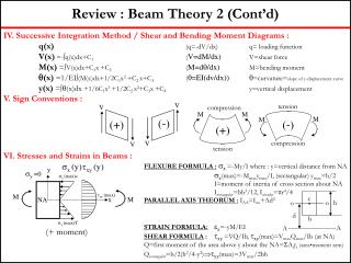
7.3 SOME BASIC DEFINITIONS In order to understand the five steps mentioned in section 7.3, some words need to be defined and relevant derivations made. 7.3.1 Stiffness and Carry-over Factors Stiffness = Resistance offered by member to a unit displacement or rotation at a point, for given support constraint conditions MB A clockwise moment MA is applied at A to produce a +ve bending in beam AB. Find A and MB. MA A B A A RA RB L E, I – Member properties
Using method of consistent deformations MA A fAA B B L L A A 1 Applying the principle of consistent deformation, Stiffness factor = k = 4EI/L
Considering moment MB, MB + MA + RAL = 0 MB = MA/2= (1/2)MA Carry - over Factor = 1/2 7.3.2 Distribution Factor Distribution factor is the ratio according to which an externally applied unbalanced moment M at a joint is apportioned to the various members mating at the joint + ve moment M M B MBC C A A MBA C B I2 L2 I1 L1 MBD I3 L3 At joint B M - MBA-MBC-MBD = 0 D D
7.3.3 Modified Stiffness Factor The stiffness factor changes when the far end of the beam is simply-supported. MA A A B L RA RB As per earlier equations for deformation, given in Mechanics of Solids text-books.
7.4 SOLUTION OF PROBLEMS - 7.4.1 Solve the previously given problem by the moment distribution method 7.4.1.1: Fixed end moments 7.4.1.2 Stiffness Factors (Unmodified Stiffness)
7.4.1.5 Computation of Shear Forces 10 kN/m 15 kN/m 150 kN B C A D I I I 3 m 3 m 8 m 8 m
7.4.1.5 Shear Force and Bending Moment Diagrams 52.077 75.563 2.792 m 56.23 27.923 74.437 3.74 m 63.77 S. F. D. Mmax=+38.985 kN.m Max=+ 35.59 kN.m 126.704 31.693 35.08 48.307 3.74 m -69.806 84.92 98.297 2.792 m -99.985 -96.613 B. M. D
Simply-supported bending moments at center of span Mcenter in AB = (15)(8)2/8 = +120 kN.m Mcenter in BC = (150)(6)/4 = +225 kN.m Mcenter in AB = (10)(8)2/8 = +80 kN.m
Problem: Draw the shear force, bending moment and elastic diagram for the continuous beam shown in fig. by MDM due to settlement of 12 mm downward and a clockwise rotation of 0.002 rad at support D. Given data I= 200X10-5 m4 and E=200X106KN/m2
Settlement: MCD MDC * ∆ * 0.012 800 KN-m
Rotation: MDC *DC * 0.012 533.33 KN-m MCDMDC KN-m
FIXED END MOMENT: MDC =-800 KN-m MDC =+533.33 KN-m MDC=-266.67 KN-m MCD =-800 KN-m MCD =+266.66 KN-m MCD=-533.33 KN-m
Stiffness Factors: KAB = KBA = KBC = KCB = KCD=KDC= = = 0.667EI
Distribution Factors: DFAB== DFBA== DFBC== DFCB== DFCD== DFDC==
Reaction Finding:Consider member AB MA= 0 (+)=> -RB1*6 – 61.583 + 0 = 0 => RB1= -10.26 KN RB1= 10.26 KN(↓)∑Fy = 0(↑+)=> RA + RB1 = 0 RA= 10.26 KN
Consider member BC ∑MB = 0 (+)=> -RC1*6 + 246.28 + 61.562 = 0RC1= 51.307 KN∑Fy = 0(↑+)=> RC1 + RB2 = 0=> RB2= -51.307 KN RB2= 51.307 KN(↓)
Consider member CD ∑MC = 0 (+)=> -RD*6 -123.145 -246.28 = 0=> RD= -61.57 KN RD = 61.57 KN(↓)∑Fy = 0(↑+)=> RC2 + RD = 0RC2= 61.57 KN
Actual Reaction RA= 10.26 KNRB = RB1 + RB2 = -10.26 -51.307 = 61.567 KN(↓)RC = RC1 + RC2 = 51.307 + 61.57 = 112.87 KNRD = 61.57 KN(↓)
Analyzing the rigid frame from figure using moment distribution method without sidesway. 10k B D C I I 10' A 6' 10' Solution: F.E.M due to the applied load: MBD = +(10×6) = +60 k-ft 32
Stiffness: KAB = KBA = (4EI/L)AB = (4EI/L)BA = (4 × E × 3I)/10 = 12EI / 10 = 1.2EI KBC = KCB = (4EI/L)BC = (4EI/L)CB = (4 × E × I)/10 = 0.4EI KBD = KDB = O
Distribution Factors: DFAB = KAB/(KAB + Kwall) = 1.2KI/(1.2EI + α) = 0 DFBA = KBA/(KBA + KBC + KBD) =1.2EI/(1.2EI + 0.4EI + 0) = 0.75 DFCB = KCB/(KCB + Kwall) = 0 DFBC = KBC/(KBC + KBA + KBD) = 0.4EI/(0.4EI + 1.2EI + 0) = 0.25 DFBD = DFDB = 0
10k B 7.5 D C 15 60 45 10' 22.5 A 6' 10'
10K B D 60 RB1 = 10k 6' For DB Span: RB1 = 10K
RB2 = 6.75k B 45 10' 22.5 A RA = 6.75k For AB Span: ∑MB = 0 ( +) • RA × 10 – 45 – 22.5 = 0 ... RA = 6.75 k ∑ Fx = 0 ( +) • RB2 – RA = 0 ... RBh = 6.75 K
7.5 B C 15 RC = 2.25k RB3 = 2.25k 10' For span BC: ∑MB = 0 ( +) • RC × 10 – 7.5 – 15 = 0 ... RC = 2.25 k ∑FX = 0 ( +) • RB2 – RC = 0 ... RB2 = 2.25 k
2.25 2.25 B D C 6.75 10 6.75 A SFD RA = 6.75 k RBh = 6.75 k RB =10k + 2.25 k = 12.25k RC =2.25 k RD = -10k
MAB = - 22.5 MBA = - 45 MBD = +60 MBC = -15 MCB = - 7.5 7.5 + 45 B D C - 15 60 + - A 22.5 BMD
Some Definitions of MDM: • Stiffness Factor: is defined as the moment at the near end to cause a unit rotation at the near end when the far end is fixed. That means how many load required for one unit deflection. • Carry-over factor: is defined as the ratio of the moment at the fixed far end to the moment at the rotation near end.(the number + 0.5 is the carry over factor) • Distribution factor: which may be defined as the fractions by which the total unbalanced at the joint is to be distributed to the member ends meeting at the joint.
Condition of sidesway: • Unsymmetrical 2-D frame in both direction • Unsymmetrical cross sectional properties • Unsymmetrical loading condition • Unsymmetrical support settlement and rotation • Symmetrical frame with symmetrical cross-sectional properties and symmetrical vertical loading but joint translation due to lateral loading
Steps of Solution: • Step-01:Find fixed end moment due to applied load • Step-02:Find fixed end moment due to sidesway • Step-03:Find stiffness factors • Step-04:Find distribution factors • Step-05: Table of finding moment due to applied load and sidesway • Step-06: Find the support reaction • Step-07: Calculate the total moment using factor (K) • Step-08: Draw SFD,BMD and Elastic Curve
24k B C A 3I 3I 8’ 2I 2I F 16’ 20’ 2I E PROBLEM: Analyze the rigid frame shown in figure-01 by the Moment Distribution Method(MDM). Draw shear and Moment diagrams. Sketch the deformed structure. D 8’ 8’ 16’ Fig-01
Step- 01: Fixed End Moment due to Applied load 24k B C A 3I 3I MBA MAB 8’ 2I 2I 16’ 20’ 2I F E D 8’ 8’ 16’ Fig-02
Step -02: Fixed End Moment due to Sides ways ∆ ∆ B A MAD MBE ∆ C 2I MCF 2I 16 ´ 20 ´ 8' 2I MFC MEB F E MDA D Fig-03