Continuous Projection for Fast L1 Reconstruction
540 likes | 756 Vues
Continuous Projection for Fast L1 Reconstruction. Reinhold Preiner* Oliver Mattausch† Murat Arikan* Renato Pajarola† Michael Wimmer*. * Institute of Computer Graphics and Algorithms, Vienna University of Technology † Visualization and Multimedia Lab, University of Zurich.

Continuous Projection for Fast L1 Reconstruction
E N D
Presentation Transcript
Continuous Projection for Fast L1 Reconstruction Reinhold Preiner* Oliver Mattausch† Murat Arikan* Renato Pajarola† Michael Wimmer* * Institute of Computer Graphics and Algorithms, Vienna University of Technology † Visualization and Multimedia Lab, University of Zurich
Dynamic Surface Reconstruction Input (87K points)
Dynamic Surface Reconstruction Online L2 Reconstruction Input (87K points)
Dynamic Surface Reconstruction Weighted LOP (1.4 FPS) Online L2 Reconstruction Input (87K points)
Dynamic Surface Reconstruction Our Technique (10.8 FPS) Online L2 Reconstruction Input (87K points)
Recap: Locally Optimal Projection • LOP [Lipman et al. 2007], WLOP [Huang et al. 2009] Attraction
Recap: Locally Optimal Projection • LOP [Lipman et al. 2007], WLOP [Huang et al. 2009] Attraction
Recap: Locally Optimal Projection • LOP [Lipman et al. 2007], WLOP [Huang et al. 2009] Attraction
Recap: Locally Optimal Projection • LOP [Lipman et al. 2007], WLOP [Huang et al. 2009] Attraction
Recap: Locally Optimal Projection • LOP [Lipman et al. 2007], WLOP [Huang et al. 2009] Repulsion
Recap: Locally Optimal Projection • LOP [Lipman et al. 2007], WLOP [Huang et al. 2009]
Recap: Locally Optimal Projection • LOP [Lipman et al. 2007], WLOP [Huang et al. 2009]
Recap: Locally Optimal Projection • LOP [Lipman et al. 2007], WLOP [Huang et al. 2009]
Performance Issues • Attraction: performance strongly depends on the # of input points
Acceleration Approach • Reduce number of spatial components! • Naïve subsampling information loss
Our Approach • Model data by Gaussian mixture fewer spatial entities
Our Approach • Model data by Gaussian mixture fewer spatial entities • Requires continuous attraction of Gaussians ?
Our Approach • Model data by Gaussian mixture fewer spatial entities • Requires continuous attraction of Gaussians Continuous LOP (CLOP)
CLOP Overview Compute Gaussian Mixture Input Solve Continuous Attraction
CLOP Overview Compute Gaussian Mixture Input Solve Continuous Attraction
Gaussian Mixture Computation initialize each point with Gaussian • Hierarchical Expectation Maximization:
Gaussian Mixture Computation initialize each point with Gaussian • Hierarchical Expectation Maximization:
Gaussian Mixture Computation initialize each point with Gaussian • Hierarchical Expectation Maximization:
Gaussian Mixture Computation initialize each point with Gaussian • Hierarchical Expectation Maximization:
Gaussian Mixture Computation initialize each point with Gaussian pick parent Gaussians • Hierarchical Expectation Maximization:
Gaussian Mixture Computation initialize each point with Gaussian pick parentGaussians EM: fit parents based on maximum likelihood • Hierarchical Expectation Maximization:
Gaussian Mixture Computation initialize each point with Gaussian pick parentGaussians EM: fit parents based on maximum likelihood Iterate over levels • Hierarchical Expectation Maximization: CLOP (8 FPS)
Gaussian Mixture Computation • Conventional HEM: blurring CLOP (8 FPS)
Gaussian Mixture Computation • Conventional HEM: blurring
Gaussian Mixture Computation • Conventional HEM: blurring • Introduce regularization
Gaussian Mixture Computation • Conventional HEM: blurring • Introduce regularization
CLOP Overview Compute Gaussian Mixture Input Solve Continuous Attraction
Continuous Attraction from Gaussians Discrete K q p1 p2 p3
Continuous Attraction from Gaussians Discrete K q Continuous Θ1 Θ2
Results Weighted LOP Continuous LOP
Results Weighted LOP Continuous LOP
Results Weighted LOP Continuous LOP
Performance 7x Speedup Weighted LOP Continuous LOP Input (87K points )
Accuracy WLOP CLOP
Accuracy Gargoyle