Download
1 / 28
370 likes | 657 Vues
Lectures 22 & 23: DETERMINATION OF EXCHANGE RATES. Building blocs - Interest rate parity - Money demand equation - Goods markets Flexible-price version: monetarist/Lucas model - derivation - applications: hyperinflation; speculative bubbles

E N D
Lectures 22 & 23: DETERMINATION OF EXCHANGE RATES • Building blocs • - Interest rate parity- Money demand equation- Goods markets • Flexible-price version: monetarist/Lucas model - derivation - applications: hyperinflation; speculative bubbles • Sticky-price version: Dornbusch overshooting model • Forecasting
Motivations of the monetary approach Because S is the price of foreign money (in terms of domestic), it is determined by the supply & demand for money (foreign vs. domestic). Key assumption: Expectedreturns are equalizedinternationally. • Perfect capital mobility => speculators are able to adjust their portfolios quickly, to reflect their desires; • + There is no exchange risk premium.=> UIP holds: Key results: • S is highly variable, like other asset prices. • Expectations are key.
Building blocks Interest rate parity + Money demand equation + Flexible goods prices => PPP => monetarist or Lucas models. or+ Slow goods adjustment => sticky prices => Dornbusch overshooting model.
INTEREST RATE PARITY CONDITIONS • Covered interest parityin one locationholds perfectly. • Covered interest parityacross countriesholds to the extent capital controls and other barriers are low. • Uncovered interest parityholds if risk is unimportant, which is hard to tell in practice. • Real interest paritymay hold in the long runbut not in the short run .
TWO KINDS OF MONETARY MODELS • Goods prices perfectly flexible • => Monetarist/ Lucas model (2) Goods prices sticky => Dornbusch overshooting model
MONETARIST/LUCAS MODEL • PPP: • + Money market equilibrium:1/ • Experiment 1a:M => S in proportion 1b:M* => S in proportion Why? Increase in supply of foreign money reduces its price. 1/ The Lucas version derives Lfrom optimizingbehavior,rather than just assuming it.
Experiment 2a:Y => L => S . 2b:Y* => L * => S . Why? Increase in demand for foreign money raises its price. Experiment 3:pe => i => L => S Why? i-i* reflects expectation of future depreciation se(<= UIP), due (in this model) to expected inflation pe.So investors seek to protect themselves: shift out of domestic money.
ILLUSTRATIONS OF THE IMPORTANCEOF EXPECTATIONS (se): • Effect of “News”: In theory, S jumps when, and only when, there is new information, e.g., re: monetary fundamentals. • Hyperinflation:Expectation of rapid money growth and loss in the value of currency => L => S, even ahead of the actual inflation & depreciation. • Speculative bubbles:Occasionally a shift in expectations, even if not based in fundamentals, can cause a self-justifying movement in L and S. • Target zone: If the band is credible, speculation can stabilize S, pushing it away from the edges even ahead of intervention. • Random walk: Information about the future already incorporated in today’s price (but does not imply zero forecastability of RW).
Effect of News: In 2002, when Lula pulled ahead of the incumbent party in the polls, fearful investors sold Brazilian reals.
The world’s most recent hyperinflation: Zimbabwe, 2007-08 Inflation peaked at 2,600% per month.
The central bank monetized government debt. The driving force?Increase in the money supply:
The exchange rate S increased along with the price level P. Both P & S rose far more than the money supply. Why? When the ongoing inflation rate is high, the demand for money is low in response.For M/P to fall, P must go up more than M.
Limitations of the monetarist/Lucas modelof exchange rate determination No allowance for SR variation in:The real exchange rate QThe real interest rate r . One approach: International versions of Real Business Cycle models assume all observed variation in Q is due to variation in LR equilibrium (and r is due to ), in turn due to shifts in tastes, productivity. But we want to be able to talk about transitory deviations of Q from (and r from ), arising for monetary reasons. => Dornbusch overshooting model.
From Lecture 10: Sticky goods prices => autoregressive pattern in real exchange rate. Adjustment ≈ 25% p.a.(though you need 200 years of data to see it) 1980Thatcher appreciation 1925 ₤ return to gold 1990: ₤ enteredEMS 1931, 49, 69₤ devaluations 1992: ₤ leftEMS UK inflation duringBretton Woods era
DORNBUSCH OVERSHOOTING MODEL PPP holds only in the Long Run, for . In the SR, S can be pulled away from . • Consider an increase in real interest rate r i -pee.g., due to M contraction, as in UK1980, US1982, Japan1990, or Brazil2011. • Domestic assets more attractive • Appreciation: Suntil currency “overvalued” relative to When seis large enough to offset i- i*, that is the overshooting equilibrium . => investors expect future depreciation. t • S
Then, dynamic path: • high r and high currency => low demand for goods(as in Mundell-Fleming model) • => deflation, or low inflation • => gradually rising M/P • => gradually falling i & r • => gradually depreciating currency. • In LR, neutrality: • P and S have changed in same proportion as M • => M/P, S/P, r and Y back to LR equilibria.
The experiment in the original Dornbusch article:a permanent monetary expansion. • => fall in real interest rate, r i - Δpe=> domestic assets less attractive => depreciation: S , • until currency “undervalued” relative to .=> investors expect future appreciation. • When - Δse offsets i-i*, that is the overshooting equilibrium. • Then, dynamic path: low r and low currency • => high demand for goods => high inflation • => gradually falling M/P => gradually rising i & r • => gradually appreciating currency. • Until back to LR equilibrium. • S t
The Dornbusch model ties it all together: • In the short run, it is the same as the Mundell-Fleming model, • except that se is what lets interest rates differ across countries, • rather than barriers to the flow of capital. • In the long run, it is the same as the monetarist/Lucas model • The path from the short run to the long run is driven by the speed of adjustment of goods prices, • which also drives the path from flat to steep AS curves. • Estimated adjustment from the PPP tests ≈ 25% or 30% per year.
SUMMARY OF FACTORS DETERMINING THE EXCHANGE RATE (1) LR monetary equilibrium: (2) Dornbusch overshooting:SR monetary fundamentals pull S away from ,(in proportion to the real interest differential). (3) LR real exchange rate can change, e.g., Balassa-Samuelson or oil shock. (4) Speculative bubbles.
TECHNIQUES FOR PREDICTING THE EXCHANGE RATE Models based on fundamentals • Monetary Models • Monetarist/Lucas model • Dornbusch overshooting model • Other models based on economic fundamentals • Portfolio-balance model… Models based on pure time series properties • “Technical analysis” (used by many traders) • ARIMA or other time series techniques (used by econometricians) Other strategies • Use the forward rate; or interest differential; • random walk (“the best guess as to future spot rate is today’s spot rate”)
Appendices • Appendix 1: The Dornbusch overshooting graph • Appendix 2: Example: The dollar • Appendix 3: Testing bias in the forward discount
Appendix 1 In the instantaneous overshooting equilibrium (at C), S rises more-than-proportionately to M to equalize expected returns. M↑ => i ↓ => S ↑ while P is tied down. i gradually rises back toi* Excess Demand(at C)causes P to rise over time until reaching LR equilibrium (at B). i<i*
Appendix 2:The example of the $ (trade-weighted, 1974-2006) • Compute real interest rate in US & abroad(Fig. a) • Differential was • negative in 1979, • rose sharply through 1984, and • then came back down toward zero. • Real value of the dollar followed suit(Fig. b) • But many fluctuations cannot be explained, even year-long • Strongest deviation: 1984-85 $ appreciation, & 2001-02. • Speculative bubble?
US real interest rate peaked in 1984. due to Volcker/Reagan policy mix. US real interest rate < 0 in late 70s (due to high inflatione).
Real $ rose with monetary fundamentals. & then beyond, in 1984-85. & again 2001-02 (esp. vs. €). Real interest differential peaked in 1984 . ¥ in 1995 may have been another bubble
Appendix 3 • Testing the hypothesis that the forward rate F isan unbiased predictor of future S • Is the interest differential an unbiased predictor of the future rate? • Testing unbiasedness tests UIP together with rational expectations. • Given C.I.P. (i-i*=fd), it’s the same question as whether the forward discount fd is unbiased; • but we can test it at longer horizons. • The predictions seem to get better at longer horizons. • One motive for studying the bias. • If investors treat domestic & foreign bonds as imperfect substitutes, forex intervention has an effect even if sterilized. • The criterion for perfect substitutability: Uncovered interest parity
IS THE FORWARD RATE AN UNBIASED FORECASTER FOR THE FUTURE SPOT RATE? Regression equation: st+1 = + (fdt) + εt+1 Unbiasedness hypothesis: = 1 Random walk hypothesis: = 0 Usual finding: << 1. (Sometimes ≈ 0, or even <0.) => fd is biased Possible interpretations of finding: 1) Expectations are biased (investors do not determine se optimally), or else2) there is an exchange risk premium (fd - se 0)