Download

1 / 46
511 likes | 2.42k Vues
Populations and Samples. Dr David Field. General Information. This lecture contains material that is crucial for understanding the rest of the course read the text book important sections are indicated by, e.g. go to the workshop download the lecture

E N D
Populations and Samples Dr David Field
General Information This lecture contains material that is crucial for understanding the rest of the course • read the text book • important sections are indicated by, e.g. • go to the workshop • download the lecture • make use of the university maths support service • Specialist statistics tutor available every Wednesday afternoon in term time from 2.00pm-4.00pm • Alternatively, in a form with your question on the website and get a reply by email • http://www.reading.ac.uk/mathssupport/ 2.5.2
Populations and samples • At the end of this lecturewe will be able to make statements of the form • “We measured the number of hours slept per night of a sample of 50 students in the UK. The mean number of hours slept was 7.2. We can be 95% confident that the population mean lies between 6.8 and 7.6 hours of sleep per night.” • We will aim to understand the logic underlying the confidence interval around the mean in the above statement • This is based on the properties of normal distributions and sampling distributions
Populations and samples 2.3 • If we weighed every adult domestic cat in the UK we would be able to calculate the population mean weight and the population SD • other populations of interest might be engineering students or amateur cricketers or cars • Measuring the whole population is expensive and impractical, and so scientists invariably measure only a fraction of the population of interest, using sampling • The aim of the sampling procedure is to obtain as good an estimate of the unknown true population statistics as possible • This requires the relationship between the sample you have and the unknown population to be quantified • If I weigh 100 cats, how confident can I be that my observed mean is close to the unobservable population mean?
Representative and unrepresentative samples • We can only assess the relationship between a sample and an unobservable population if the sample is representative of the target population • This is an issue of study design, but it determines how broadly we can interpret our numeric statistics • If a sample of engineering students was selected exclusively from Oxford University then measures obtained from it might not be an accurate reflection of engineering students in general • There are a number of ways to obtain a representative sample, the simplest case being random selection from the entire population
What does random mean? • Each time you sample a single case, every member of the underlying population had an equal chance of being selected • The classic case is rolling an unbiased dice • Each time the die is rolled you have an equal chance of the result being 1,2,3,4,5, or 6 • There are no history effects! • If you rolled 600,000 dice and recorded the results you would end up with very close to 100,000 occurrences of each outcome • What would the frequency histogram of this data look like? • In Psychology we often use opportunity samples and treat them as if they were random samples from a target population
Key concept: the normal distribution 1.7.1 • Values close to the mean of a variable are often more frequent than values far from the mean • This is true of the height of adults, • It is not true of rolling a dice repeatedly • When true, and if you sample randomly from the population, this produces a bell shaped frequency histogram • Many psychological variable are normally distributed, e.g. IQ • in the case of the IQ test, it is designed to be like that • Normal distributions can be visualised using frequency histograms just like the ones from Lecture 1
UK cats Mean 5 Kg SD 0.8 Kg Carl Frederick Gaus (1777-1855)
Curve shape is independent of sample size UK cats Mean 5 Kg SD 0.8 Kg
The standard deviation - revision • The sum of the squared deviations is 64 • The mean deviation (variance) is therefore 64 /(6 – 1) = 12.8 • Square rooting the variance returns it to the original measurement units of the variable • Therefore the SD is 3.57 pints
Greek cats Mean 3.55 Kg SD 0.4 Kg UK cats Mean 5.0 Kg SD 0.8 Kg
A Greek cat weighing 3.95 Kg and a British cat weighing 5.8 Kg are clearly different from each other in important ways, including their weight • But, to a statistician, they are identical in one important respect: • they occupy the same position in their respective sample distributions • relative to their sample means they are both equally “unusual” occurrences • Both can be described by “Mean + 1SD” • If you randomly select 1 cat from the 10,000 Greek and the 10,000 British cats then the probability of sampling a 5.8 Kg British cat is equal to the probability of sampling a 3.95 Kg Greek cat
UK cats Mean 5.0 Kg SD 0.8 Kg
6800 Greek cats UK cats Mean 5.0 Kg SD 0.8 Kg
Recall the student sleep example from the start of the lecture, and the 95% confidence interval around the mean number of hours slept? • For any population that is normally distributed 95% of all scores will fall within 1.96 SD either side of the mean • This means that if you randomly select one case, it’s score is 95% likely to fall within 1.96 SD of the mean • This fact is an important part of the story
The standard normal distribution and z scores 1.7.4 • The family of normal distributions has an infinite number of members, each defined by a unique combination of mean and SD • There is one particular normal distribution, called the standard normal distribution, which has a special status • It has a mean of 0 • It has a SD of 1
The standard normal distribution and z scores • One useful thing about the standard normal distribution is that scores from any other normal distribution can be converted into scores on the standard normal distribution • The converted scores are called z scores • The new scores loose their original units (e.g. Kg), and are now expressed in units of SD • This is useful for comparing between samples • If you know the z score for a Greek cat and for a British cat you see directly which cat is a relatively heavier example of it’s own population
Calculating z scores • z = (score – sample mean) / SD of sample • z score for a British cat weighing 4.7 Kg • (4.7 – 5.0) / 0.8 = -0.62 • z score for a Greek cat weighing 4.7 Kg • (4.7 – 3.5) / 0.4 = 2.88 • The Greek cat is a very large cat • The British cat is fairly typical, perhaps slightly on the small side
What happens when the sample is small? • In Psychology we usually work with small samples, and we often have little idea of the underlying population parameters • With a small sample, you can still calculate a mean and an SD, although the sample might be too small to assess whether the underlying population is normally distributed • Lying at the heart of statistics is the question of the relationship between populations and samples • To explore this, we can use examples where population parameters are known
Population: Mean 5 Kg SD 0.8 Kg Sample of 10: Mean 4.6 Kg SD 0.7 Kg
Confidence in the sample mean 2.5 • Given a sample, I can produce a sample mean • Statistics is about describing the relationship between measured samples and underlying populations • A statistician will ask how good the sample mean is as an indicator of the population mean • If you have a large and representative sample, then the sample mean is such a good estimate of the population mean that it can be used interchangeably • But often we have a small sample, and no population data (or large sample) to compare it with • We can use the cats example, treating the full sample of 10,000 as the population, to explore the relationship between small samples and the population • A key point is that the mean of a large sample is more likely to lie close to the population mean than the mean of a small sample
Quantifying confidence in the sample mean • The sample mean is a point estimate of the population mean • If we collected a second random sample we would have two different point estimates of the population mean • By definition, they can’t both be correct • This situation implies an underlying continuum on which point estimates can lie • A continuum can be thought of as a curve plotted on a graph, like the normal distributions you saw earlier • In statistics, we aim to convert the sample point estimate into an interval estimate • This is a range on the underlying continuum • We want to be able to say that given the sample, the population mean lies somewhere between X and Y • We will have to be content to say that we are 95% sure
Where each black line crosses the x axis represents a separate point estimate of the population mean Mean 5 Kg SD 0.8 Kg The blue line is a visually judged interval estimate of the population mean given the 10 samples
Sampling distributions 2.5.1 • Each sub-sample of 10 cats has a mean weight and SD that is slightly different from the full population of 10,000 • Individual samples of 10 are often not normally distributed • Imagine collecting 100 separate sub-samples of 10 cats, and producing 100 sample means • The mean of the 100 sample means would be an excellent estimate of the population mean • It is possible to plot a frequency histogram of the 100 obtained sample means
Sampling distributions • The frequency histogram of the 100 samples of 10 will itself be normally distributed • This means the distribution can be defined by its mean and SD • More generally, if you collect a sample, then theoretically speaking there is an underlying population of samples, of which yours is just one case • The population of sample means is normally distributed
Sampling distributions • In the frequency histogram of the original sample, each case was a single cat • In the corresponding sampling distribution, each case is the mean weight of (10) cats selected randomly from the cat population • A key property of sampling distributions is that provided the individual samples have N >= 30 they are ALWAYS normally distributed • even if the actual population is skewed (e.g. reaction time) • or bimodal • if population is normal sampling distribution will also be normal for small samples < 30
The black curves are frequency histograms of the means of samples randomly selected from the pink population distribution
Populations and samples • If we had enough samples to plot a sampling distribution, then for one sample we could assess exactly how close it is to the population mean (mean of the sampling distribution) • But what if we only have one sample? • With only one sample, because sampling distributions are normally distributed we still know that the mean of the single sample is 95% likely to fall within 1.96 SD either side of the mean of a theoretical sampling distribution • Avoid confusion: • the mean of a sampling distribution IS equal to the population mean • the SD of a sampling distribution is NOT equal to the SD of the population
Standard error (SE) 2.5.1 • In statistics, the standard deviation of a sampling distribution is given a different name to distinguish it from the standard deviation of a single sample or the standard deviation of a population • It is called the standard error (SE) • Its name contains the word “error” because statisticians use it to estimate measurement error
Standard error (SE) • We can be 95% sure that a sample mean will lie within + / - 1.96 SE of the mean of the distribution of sample means • this provides the 95% confidence interval from the example about how long students sleep given at the start of the lecture • 7.2 hours – 0.4 hours (1.96 * SE) = 6.8 hours is the lower bound • 7.2 hours + 0.4 hours (1.96 * SE) = 7.6 hours is the upper bound • But at the moment we have only seen how to calculate the SE if you have collected a huge number of samples of a specific size • Therefore, the problem to solve is how to find the SE from a single sample • The starting point for solving this problem is the fact that the SE of the sampling distribution shrinks as the individual samples making up the distribution increase in size • This in turn is because the mean of a large sample is more likely to be close to the population mean than the mean of a small sample
The SE of the sampling distribution is smaller when the individual samples making up the distribution are larger
Standard error and confidence intervals • The previous slide illustrates that the confidence interval around a sample mean will be smaller if the sample size is bigger • smaller confidence intervals imply more accurate and therefore more useful measurements • There is a lawful relationship between the sample size and the SE of the resulting sampling distribution • the SE is halved when the sample size is quadrupled • The SE is also dependent upon the SD of the population the samples were drawn from • the SE is smaller when the population SD is smaller • the SD of a single sample can be used as an estimate of the population SD
Standard error and confidence intervals • This relationship between the SE, sample size, and the SD is captured in the following formula The sample SD is used as an estimate of the population SD SD of the sample = SE Sample size The value of this doubles every time sample size quadruples. E.g.Root 4 = 2, Root 16 = 4, Root 64 = 8
Standard error and confidence intervals • Standard error (SE) = sample SD / square root of sample size • For the small sample of 10 UK cats we observed a SD of 0.7 kg • 0.7 / square root of 10 (3.16) = 0.22 Kg • One more step is required to arrive at a 95% confidence interval • The standard error is 1SD of the sampling distribution • What proportion of samples have means that lie within 1SE of the mean of the sampling distribution?
It is 68% likely that the population mean falls within 1 standard error above or below the sample mean
Standard error and confidence intervals 2.5.2 • By convention, we usually want to make the statement that we are 95% certain that the population mean lies between X and Y • Therefore, we use the properties of normal distributions, which tells us that 95% of all samples in the sampling distribution of the mean fall within 1.96 SE of the mean • The confidence interval we give around the sample mean is 1.96 * SE either side of the mean
Standard error and confidence intervals • The mean of the 10 cat small sample was 4.6Kg (SD 0.7). This gives a standard error of 0.22 Kg • Confidence interval = 1.96 * 0.22 = 0.43 Kg either side of the mean • “We measured the weight of 10 adult cats in the UK. The mean weight of the sample was 4.6 Kg. We can be 95% confident that the population mean weight of adult cats in the UK lies between 4.16 and 5.03 Kg.” • The mean of the population of 10,000 cats was 5.0 Kg, and we can see that the above statement is true (but only just in this case!)
Standard error and confidence intervals • It is important to remember that we accept a 5% risk that the interval estimate is wrong, and the population mean does not lie within the range of values it defines • This is the risk that the sample we have is located in one of the two tails of the underlying sampling distribution • Imagine we draw a second sample, this time of 40 UK adult cats, from the population of 10,000 • This time, we obtain a mean weight of 4.87 Kg, with a SD of 0.84 Kg • This SD is bigger than the SD of the small sample, which was 0.7, so in a sense this sample is showing greater variation
Standard error and confidence intervals • You might expect that the SE and confidence interval will also be larger for this sample • But, because the SE formula involves dividing by the square root of the sample size it turns out that this is not the case • Standard error is 0.835 / square root 40 (6.32) = 0.13 • Confidence interval is 0.13 * 1.96 = 0.258 Kg either side of the mean • Confidence interval for the small sample was 0.43 Kg either side of the mean
long tail short tail Meaning of SD and Z scores?