Overview of Control System Design
320 likes | 563 Vues
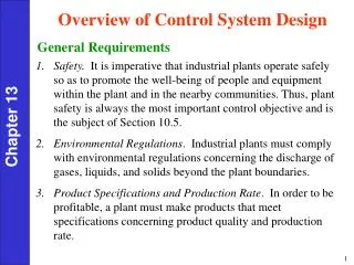
Overview of Control System Design . General Requirements.

Overview of Control System Design
E N D
Presentation Transcript
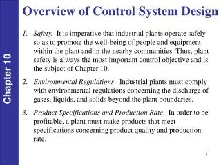
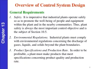
Overview of Control System Design General Requirements • Safety. It is imperative that industrial plants operate safely so as to promote the well-being of people and equipment within the plant and in the nearby communities. Thus, plant safety is always the most important control objective and is the subject of Section 10.5. • Environmental Regulations. Industrial plants must comply with environmental regulations concerning the discharge of gases, liquids, and solids beyond the plant boundaries. • Product Specifications and Production Rate. In order to be profitable, a plant must make products that meet specifications concerning product quality and production rate. Chapter 13
Economic Plant Operation. It is an economic reality that the plant operation over long periods of time must be profitable. Thus, the control objectives must be consistent with the economic objectives. • Stable Plant Operation. The control system should facilitate smooth, stable plant operation without excessive oscillation in key process variables. Thus, it is desirable to have smooth, rapid set-point changes and rapid recovery from plant disturbances such as changes in feed composition. Chapter 13
Steps in Control System Design After the control objectives have been formulated, the control system can be designed. The design procedure consists of three main steps: • Select controlled, manipulated, and measured variables. • Choose the control strategy (multiloop control vs. multivariable control) and the control structure (e.g., pairing of controlled and manipulated variables). • Specify controller settings. Chapter 13
Control Strategies • Multiloop Control: Each output variable is controlled using a single input variable. • Multivariable Control: • Each output variable is controlled using more than one input variable. Chapter 13
13.1 Degrees of Freedom for Process Control • The important concept of degrees of freedom was introduced in Section 2.3, in connection with process modeling. • The degrees of freedom NF is the number or process variables that must be specified in order to be able to determine the remaining process variables. • If a dynamic model of the process is available, NF can be determined from a relation that was introduced in Chapter 2, Chapter 13 where NV is the total number of process variables, and NEis the number of independent equations.
For process control applications, it is very important to determine the maximum number of process variables that can be independently controlled, that is, to determine the control degrees of freedom, NFC: Definition. The control degrees of freedom, NFC, is the number of process variables (e.g., temperatures, levels, flow rates, compositions) that can be independently controlled. Chapter 13 • In order to make a clear distinction between NF and NFC, we will refer to NF as the model degrees of freedom and NFC as the control degrees of freedom. • Note that NF and NFC are related by the following equation, where NDis the number of disturbance variables (i.e., input variables that cannot be manipulated.)
General Rule. For many practical control problems, the control degrees of freedom NFC is equal to the number of independent material and energy streams that can be manipulated. Example 13.1 Chapter 13 Determine NF and NFC for the steam-heated, stirred-tank system modeled by Eqs. 2-50 – 2-52 in Chapter 2. Assume that only the steam pressure Ps can be manipulated. Solution In order to calculate NF from Eq. 13-1, we need to determine NVand NE. The dynamic model in Eqs. 2-50 – 2-52contains three equations (NE = 3) and six process variables (NV = 6): Ts, Ps, w, Ti, T, and Tw. Thus, NF = 6 – 3 = 3.
Chapter 13 Figure 13.1 Two examples where all three process streams cannot be manipulated independently.
Stirred-Tank Heating Process Chapter 13 Figure 2.3 Stirred-tank heating process with constant holdup, V.
If the feed temperature Ti and mass flow rate w are considered to be disturbance variables, ND = 2 and thus NFC = 1 from Eq. (13-2). • It would be reasonable to use this single degree of freedom to control temperature T by manipulating steam pressure, Ps. Example 13.2 Chapter 13 The blending system in Fig. 13.3 has a bypass stream that allows a fraction f of inlet stream w2 to bypass the stirred tank. It is proposed that product composition x be controlled by adjusting f via the control valve. Analyze the feasibility of this control scheme by considering its steady-state and dynamic characteristics. In your analysis, assume that x1 is the principal disturbance and that x2, w1, and w2 are constant. Variations in the volume of liquid in the tank can be neglected because w2 << w1.
Chapter 13 Figure 13.3. Blending system with bypass line.
Solution • The dynamic characteristics of the proposed control scheme are quite favorable because the product composition x responds rapidly to a change in the bypass flow rate. • In order to evaluate the steady-state characteristics, consider a component balance over the entire system: Chapter 13 Solving for the controlled variable gives, • Thus depends on the value of the disturbance variable and four constants (w1, w2, x2, and w). • But it does not depend on the bypass function, f.
Thus, it is not possible to compensate for sustained disturbances in x1 by adjusting f. • For this reason, the proposed control scheme is not feasible. • Because f does not appear in (13-4), the steady-state gain between x and f is zero. Thus, although the bypass flow rate can be adjusted, it does not provide a control degree of freedom. • However, if w2 could also be adjusted, then manipulating both f and w2 could produce excellent control of the product composition. Chapter 13
Effect of Feedback Control • Next we consider the effect of feedback control on the control degrees of freedom. • In general, adding a feedback controller (e.g., PI or PID) assigns a control degree of freedom because a manipulated variable is adjusted by the controller. • However, if the controller set point is continually adjusted by a higher-level (or supervisory) control system, then neither NF nor NFC change. • To illustrate this point, consider the feedback control law for a standard PI controller: Chapter 13
where e(t) = ysp(t) – y(t) and ysp is the set point. We consider two cases: Case 1. The set point is constant, or only adjusted manually on an infrequent basis. Chapter 13 • For this situation, ysp is considered to be a parameter instead of a variable. • Introduction of the control law adds one equation but no new variables because u and y are already included in the process model. • Thus, NE increases by one, NV is unchanged, and Eqs. 10-1 and 10-2 indicate that NF and NFCdecrease by one.
Case 2. The set point is adjusted frequently by a higher level controller. • The set point is now considered to be a variable. Consequently, the introduction of the control law adds one new equation and one new variable, ysp. • Equations 13-1 and 13-2 indicate that NF and NFC do not change. • The importance of this conclusion will be more apparent when cascade control is considered in Chapter 16. Chapter 13 Selection of Controlled Variables Guideline 1. All variables that are not self-regulating must be controlled. Guideline 2. Choose output variables that must be kept within equipment and operating constraints (e.g., temperatures, pressures, and compositions).
Chapter 13 Figure 13.3 General representation of a control problem.
Guideline 3. Select output variables that are a direct measure of product quality (e.g., composition, refractive index) or that strongly affect it (e.g., temperature or pressure). Guideline 4. Choose output variables that seriously interact with other controlled variables. Guideline 5. Choose output variables that have favorable dynamic and static characteristics. Chapter 13
Selection of Manipulated Variables Guideline 6. Select inputs that have large effects on controlled variables. Guideline 7. Choose inputs that rapidly affect the controlled variables. Guideline 8. The manipulated variables should affect the controlled variables directly rather than indirectly. Guideline 9. Avoid recycling of disturbances. Chapter 13
Selection of Measured Variables Guideline 10. Reliable, accurate measurements are essential for good control. Guideline 11. Select measurement points that have an adequate degree of sensitivity. Guideline 12. Select measurement points that minimize time delays and time constants Chapter 13
Example 13.4: Evaporator Control Chapter 13 Figure 13.5 Schematic diagram of an evaporator. MVs: Ps, B and D DVs: xFand F CVs: ??
Case (a): xB can be measured Chapter 13
Case (b): ): xB cannot be measured Chapter 13
Distillation Column Control (a 5x5 control problem) Chapter 13
Challenges for Distillation Control • 1. There can be significant interaction between process variables. • 2. The column behavior can be very nonlinear, especially for high purity separations. • 3. Distillation columns often have very slow dynamics. • 4. Process constraints are important. • Product compositions are often not measured. • cf. Distillation Process Control Module (Appendix E) Chapter 13
Process Control Module: Fired-Tube Furnace Chapter 13 The major gaseous combustion reactions in the furnace are:
Process Control Module: Fired-Tube Furnace Table 3.1 Key Process Variables for the PCM Furnace Module Measured Output Variables Disturbance Variables HC outlet temperature HC inlet temperature Furnace temperature HC flow rate Flue gas (exhaust gas) flow rate Inlet air temperature O2 exit concentration FG temperature FG purity (CH4 Manipulated Variables concentration) Air flow rate FG flow rate Chapter 13
Control Objectives for the Furnace To heat the hydrocarbon stream to a desired exit temperature To avoid unsafe conditions due to the interruption of fuel gas or hydrocarbon feed To operate the furnace economically by maintaining an optimum air-fuel ratio. Chapter 13 Safety Considerations? Control Strategies?
Catalytic Converters for Automobiles Three-way catalytic converters (TWC) are designed to reduce three types of harmful automobile emissions: carbon monoxide (CO), unburned hydrocarbons in the fuel (HC) nitrogen oxides (NOx). Desired oxidation reactions (1000-1500 °F, residence times of ~ 0.05 s): Chapter 13 Desired reduction reaction:
Chapter 13 Figure 13.10 TWC efficiency as a function of air-to-fuel ratio (Guzzella, 2008).
TWC Control Strategy Chapter 13