Download
1 / 13
130 likes | 210 Vues
Explore the first analysis of Nares Strait CT-string data, revealing depth-specific patterns in pressure, salinity, and temperature. The study showcases seasonal variability, anomalies, and potential calibration issues, prompting further investigations into baroclinic transport changes. Dive into detailed profiles and tidal cycles for a comprehensive understanding.

E N D
First Analysis of theNares Strait CT-String Data Berit Rabe & Helen Johnson
o x • 6/8 CT-moorings recovered (each with 4 SBE37) • 2 missing ones are assumed to be lost, no signal • KS03: pressure sensor at 200dbar no data, • but additional pressure sensor at 80dbar • All other ones: complete 3-year record 109m
SBE37 Mooring Design: • Depth of instruments: 30m, 80m, 130m, 200m • Pressure sensors at upper and lower instrument • Flexible, made for bending due to icebergs
First evaluation of pressure data: Example: Pressure data KS05 upper instrument Red: original data Blue: 5 day low-pass filtered data Yellow: mean Green: standard deviation Pressure [dbar] Time [days since 01/01/2003]
Mean and standard deviation for low-pass filtered data • Higher variability at 30m than at 200m as expected • If pressure difference higher than 0.5dbar before and after deployment exponential fit was used
TS diagrams for KS01 and KS13 upper instruments as a function of depth. KS01 KS13
3 year salinity time series • Upper level: seasonal cycle, lowest salinity in summer • Deepening of isohalines towards Ellesmere Island at 80 and 130dbar
3 year temperature time series • Obvious seasonal variability, vertical instrument excursion and transient events... • Was winter 2003 anomalous?
Salinity Profiles * Upper 2 3 Lower x KS01 KS03 KS05 KS07 KS09 KS13 Mean S for each depth bin (when instrument is there!)
Temperature Profiles * Upper 2 3 Lower x KS01 KS03 KS05 KS07 KS09 KS13 Mean T for each depth bin (when instrument is there!)
Salinity - Julian Day 220, with 2003 and 2006 CTD profiles * Upper 2 3 Lower x KS01 - CTD 2003 KS03 KS05 KS07 KS09 KS13 - CTD 2003 - CTD 2006 (dashed) Two tidal cycles....
Temperature - Julian Day 220, with 2003 and 2006 CTD profiles * Upper 2 3 Lower x KS01 - CTD 2003 KS03 KS05 KS07 KS09 KS13 - CTD 2003 - CTD 2006 (dashed) Two tidal cycles....
What next?! • Remaining calibration issues. • Plot some sections - “snapshots” in time and mean picture in any given season. • Look at particular events (and their signature in ADCP and IPS data too). • Quantify changes in baroclinic transport on various timescales (and examine their causes). • Lots lots more.....!