Download
1 / 12
120 likes | 150 Vues
Explore a mathematical model defining the dynamics of a self-limiting population based on waste production, growth, and death rates. Analyze phase plane trajectories and limiting behavior.

E N D
A MATHEMATICAL MODELFOR ASELF-LIMITING POPULATION Glenn Ledder gledder@math.unl.edu University of Nebraska
THE CONCEPTUAL MODEL • A container holds p(t) microorganisms and a quantity w(t) of waste, with p(0)=p0«1 and w(0)=0. 2. Waste production is proportional to population. 3. In absence of waste, population growth is logistic. 4. Relative death rate increases linearly with waste amount.
THE MATHEMATICAL MODEL • Waste production is proportional to population. dw dt —–=kp w(0) = 0 • In absence of waste, population growth is • logistic. • Relative death rate increases linearly with • waste amount. dp dt p M —–=rp(1– —)–bwp p(0) =p0
NONDIMENSIONALIZATION dw dt —–=kp w(0) = 0 dp dt p M —–=rp(1– —)–bwp p(0) =p0 r b Let p=MPw=—Wτ=rt Then W′=KP W(0)=0 P′ =P(1–P–W) P(0)=P0
NULLCLINES • W is fixed when P=0 and increasing when P>0. • P is fixed when P=0 and P+W=1. P 1 W 1
The DIFFERENTIAL EQUATION for the TRAJECTORIES Trajectories satisfy the equation —– = — = ——– We can combine the differential equations to obtain the differential equation for the trajectories in the phase plane. Given W′=KP and P′ =P(1–P–W) : dP dW P′ W′ 1-P-W K
CHANGE OF VARIABLES dP dW 1-P-W K The trajectory equation, —– = ——– , is linear but not autonomous. Let Z=P+W. dZ dW Then K–— =1+K–Z. This equation is autonomous as well as linear.
PHASE LINE dZ dW K–— =1+K–Z Z=P+W. Z 1+K 1+Kis a stable equilibrium solution; however, it is not achieved because W remains finite. • P+W<1+K , and (P+W)′ > 0
TRAJECTORIES We can solve the trajectory equation to get P=1+K–W+(P0–1–K)e-W/K K=0.5 K=1.0
MAXIMUM POPULATION P=1+K–W+(P0–1–K)e-W/K The maximum population occurs when P+W=1. 1+K-P0 K P=1–W=1–Kln———
LIMITING BEHAVIOR With P0=0andP=0, we have W=(1+K)(1-e-W/K). s u-s su u-s (K,W∞) = ( ——, —— ),whereu=-ln(1-s)
EXTINCTION TIME Let T be the time (in units of 1/r) at which P=0. From W′=KP, we have W∞/K du 1+K–Ku+(P0-1-K)e-u T= —————————— 0 P0=0.01