Interquartile Range
Interquartile Range. Lecture 21 Sec. 5.3.1 – 5.3.3 Mon, Feb 23, 2004. Measuring Variation or Spread. Static view – Given a sample or a population, how spread out is the distribution?

Interquartile Range
E N D
Presentation Transcript
Interquartile Range Lecture 21 Sec. 5.3.1 – 5.3.3 Mon, Feb 23, 2004
Measuring Variation or Spread • Static view – Given a sample or a population, how spread out is the distribution? • Dynamic view – If we are taking measurements on units in the sample or population, how much will our measurements vary from one to the next?
Measures of Variation or Spread • These are two aspects of the same phenomenon. • The more variability there is in a population, the more difficult it is to estimate its parameters. • For example, it is easier to estimate the average size of a crow than the average size of a dog (thanks to selective breeding).
The Range • By far, the simplest measure of spread is the range. • Range – The difference between the largest value and the smallest value of a sample or population. • How would you expect the range of a sample compare to the range of the population?
The Range • Is the sample range a good estimator of the population range? • Would you expect it to systematically overestimate or underestimate the population range? Why? • In general, the range is a poor measure of variability since it does not take into account how the values are distributed in between the maximum and the minimum.
Percentiles • The pth percentile – A value that separates the lower p% of a sample or population from the upper (100 – p)%. • The median is the 50th percentile; it separates the lower 50% from the upper 50%. • The 25th percentile separates the lower 25% from the upper 75%.
Finding percentiles • To find the pth percentile, compute the value r = (p/100) (n + 1). • This gives the position (r = rank) of the pth percentile. • Round r to the nearest whole number. • We will use the number in that position as the pth percentile.
Finding percentiles • Special case: If r is a “half-integer,” for example 10.5, then take the average of the numbers in positions r and r + 1, just as we did for the median when n was even. • Note: The “official” procedure says to interpolate when r is not a whole number. • Therefore, by rounding, our answers may differ from the official answer.
Example • Find the 30th percentile of 5, 6, 8, 10, 15, 30. • p = 30 and n = 6. • Compute r = (30/100)(7) = 2.1 2. • The 30th percentile is 6. • The “official” answer is 6.2. • Find the 35th percentile.
Quartiles • The first quartile is the 25th percentile. • The second quartile is the 50th percentile, which is also the median. • The third quartile is the 75th percentile. • The first quartile is denoted Q1. • The third quartile is denoted Q3. • There are also quintiles and deciles.
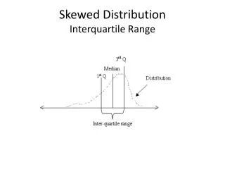
The Interquartile Range • The interquartile range (IQR) is the difference between Q3 and Q1. • The IQR is a commonly used measure of spread. • Like the median, it is not affected by extreme outliers.
Example • See Example 5.4, p. 281. • n = 20. • For Q1, r = (0.25)(21) = 5.25 5. • Q1 = 41. • For Q3, r = (0.75)(21) = 15.75 16. • Q3 = 47. • Therefore, IQR = 47 – 41 = 6.
Computing Quartiles on the TI-83 • Follow the procedure used to find the mean and the median. • Scroll down the display to find Q1 and Q3.
Computing Quartiles on the TI-83 • In our last example, the TI-83 says that • Q1 = 41 • Q3 = 46.5 • Other software might compute Q3 = 46.75.