Download
1 / 33
330 likes | 415 Vues
Exploring numerical, graphical, and algebraic approaches to limits, derivatives, and continuity in mathematics, with real-world applications and examples provided.

E N D
Chapter 3 Introduction to the Derivative 3.1 Limits: Numerical and Graphical Approaches 3.2 Limits and Continuity Limits and Continuity: Algebraic Approach 3.3 3.4 Average Rate of Change 3.5 Derivatives: Numerical and Graphical Viewpoints 3.6 The Derivative: Algebraic Viewpoint
3.1 Limits Definition of a Limit : If f (x) approaches the number L as x approaches (but is not equal to) a from both sides, then we say that f (x) approaches L as x →a (“x approaches a”) or that the limit of f (x) as x → a is L. (Note: If f(x) fails to approach a single fixed number then the limit does not exist – DNE) Rates of change are calculated by derivatives, but an important part of the definition of the derivative is something called a limit. Example:f (x) = 2 + x , What happens to f (x) as x approaches 3? The closer x gets to 3 from either side, the closer f(x) gets to 5. The limit of f(x), as x approaches 3, equals 5.
More Challenging Examples • As x gets closer to zero on either side, f (x) gets larger and larger without bound—if you name any number, no matter how large, f (x) will be even larger than that if x is sufficiently close to 0. does not exist, and because f (x) is becoming arbitrarily large, we also say that the limit diverges to So, limx→0f(x) does not exist.
Numerical & Graphical Solutions Now, Try graphing the function. x y . -1 -1/3 0 -1/2 ½ 2 1 -1 2 undefined 3 1 Examine f(x) as you approach 2 from the right and from the left Does it match your numerical findings?
Estimating Limits Graphically • Remember: • Limits must be the same from the right and from the left or they do not exist. • Try these: • Answers: 2 DNE 1 +∞ • Note: If x = a is an endpoint of the domain of f, • then only a one-sided limit is possible at x = a. • Suppose the domain of f is (– ∞, 4], then limx→4–f (x) • can be computed, but not limx→4+f (x). In this case, we • have said that limx→4f (x) is just the one-sided limit • limx→4–f (x).
An Application The percentage of U.S. Internet-connected households that have broadband connections can be modeled by where t is time in years since 2000. Find: and Thus, in the long term (as t gets larger and larger), the percentage of U.S. Internet connected households that have broadband is expected to approach 100%. Thus, the closer t gets to 0 (representing 2000) the closer P(t) gets to 8.475%, meaning that, in 2000, about 8.5% of Internet-connected households had broadband.
3.2 Limits and Continuity Recall that this graph has breaks, or discontinuities, at x = 0 and x = 1. At x = 0 limx→0f (x) does not exist because left and right limits are not the same. At x = 1, limx→1f(x) does exist (it is equal to 1), but is not equal to f(1) = 2. Functions are discontinuous at: 1. Points where the limit of the function does not exist. 2. Points where the limit exists but does not equal the value of the function. At x = –2, there is no discontinuity. limx→–2f(x) exists and equals 2 : f(–2) = 2. The function is continuousat x = -2.
Definition: Limits and Continuity Continuous Function : Let f be a function and let a be a number in the domain of f. Then f is continuous at a if a.limx→a f (x) exists, and b.limx→a f (x) = f (a). The function f is said to be continuous on its domain if it is continuous at each point in its domain. If f is not continuous at a particular a in its domain, we say that f is discontinuous at a or that f has a discontinuity at a. Thus, a discontinuity can occur at x = a if either a. limx→a f(x) does not exist, or b. limx→a f(x) exists but is not equal to f(a).
Continuous? Discontinuous? h(x)= x + 3 if x ≤ 1 5 – x if x > 1 k(x) = x + 3 if x ≤ 1 1 – x if x > 1 g(x) = 1/x if x ≠ 0 0 if x = 0 f(x) = 1/x Continuous at every Point in the domain. Note that 0 is not in The doman of f(x) Domain expanded to include 0. limx→0g(x) DNE, so Discontinuous at x = 0 g is discontinuous on its domain. Discontinuous at x = 1 limx→1k(x) does not exist (DNE) k(x) is not continuous on its domain. Continuous at every Point in the domain.
3.3 Limits: Algebraic Approach Closed-Form Functions Functions specified by combining constants, powers of x, exponential functions, radicals, logarithms, absolute values, trigonometric functions (and some other functions) into a single mathematical formula by means of the usual arithmetic operations and composition of functions. 3x2 – |x| + 1 : Closed-Form –1 if x ≤ –1 f(x) = x2 + x if –1 < x ≤ 1 NOT Closed-Form 2 – x if 1 < x ≤ 2 Every closed-form function is continuous on its domain.Thus, if f is a closed-form function and f (a) is defined, we have limx→a f (x) = f (a). Considerf(x) = 1/x where the domain is all real numbers except 0. a ≠ 0
Examples – Limit of Closed-Form Function at a Point in Its Domain • Example 1: • Note: This is a Closed-form function, and x=1 is in the domain. • Example 1 (Revisited - Another way) • : (x – 2) (x2 + 2x + 4) = (x2 + 2x + 4). So, (12 + 2(1) + 4) = 7 • (x – 2) • Example 2: • Recall that x2 – 1 = (x + 1)(x -1)
Limits at Infinity Suppose we want to compute the following limits: Solution for a and b. The highest power of x in both the numerator and denominator dominate the calculations. For instance, when x = 100,000, the term 2x2 in the numerator has the value of 20,000,000,000, whereas the term 4x has the comparatively insignificant value of 400,000. Similarly, the term x2 in the denominator overwhelms the term –1.
Limits at Infinity cont’d • c. • As x gets large, –x/ 2 gets large in magnitude but negative. • d. As x gets large, 2/(5x) gets close to zero. e. Here we do not have a ratio of polynomials. However, we know that, as t becomes large and positive, so does e0.1t, and hence also e0.1t– 20.
Limits at Infinity Continued… cont’d • f. As t → , the term (3.68)–t = in the denominator, • being 1 divided by a very large number, approaches zero. • Hence the denominator 1 + 2.2(3.68)–tapproaches • 1 + 2.2(0) = 1 as t → . THEOREM: Evaluating the Limit of a Rational Function at If f (x) has the form with the ciand diconstants (cn 0 and dm 0), then we can calculate the limit of f (x) as x → ±∞ by ignoring all powers of x except the highest in both the numerator and denominator.
Some Determinate and Indeterminate Forms are indeterminate; evaluating limits in which these arise requires simplification or further analysis. The following are determinate forms for any nonzero number k: Examples:
3.4 Average Rate of Change (Numerical) • The following table lists the approximate value of Standard and Poor’s 500 stock market index (S&P) during the period 2000–2008 (t = 0 is 2000): What was the average rate of change in the S&P over the 2-year period 2005–2007 (the period 5 t 7 or [5, 7] in interval notation); over the 4-year period 2000–2004 (the period 0 t 4 or [0, 4]); and over the period [1, 5]? Thus, the S&P increased by 300 points in 2 years, giving an average rate of change of 300/2 = 150 points per year. S&P increased at an average rate of 150 points per year.
Average Rate of Change (Graphical) Notice that this rate of change is also the slope of the line through P and Q, and we can estimate this slope directly from the graph.
Average Rate of Change of a Function Numerically and Graphically • The change in f (x) over the interval [a, b] = Change in f = f • = Second value – First value • = f (b) – f (a). • The average rate of change of f (x) over the interval [a, b] is • (Also called the “difference quotient”) Units The units of the change in f are the units of f(x). The units of the average rate of change of f are units of f(x) per unit of x. PQ is called a “Secant line” of the graph Average rate of change = Slope of PQ
Average Rate of Change (Alternative Formula) The average rate of change of f (x) over the interval [a, b] Alternative Formula: Average Rate of Change of f(x) Replace b above by a + h The average rate of change of f over the interval [a, a + h] is
Example: Average Rate of Change • You are a commodities trader and you monitor the price of gold on the New York Spot Market very closely during an active morning. Suppose you find that the price of an ounce of gold can be approximated by the function • G(t) = –8t 2 + 144t + 150 dollars (7.5 ≤ t ≤ 10.5) [t = time in hours] What was the average rate of change of the price of gold over the -hour period starting at 8:00 AM(the interval [8, 9.5])? 796 – 790 9.5 – 8 6 = $4 per hour 1.5 Gold price increased at an average rate of $4 per hour from 8am to 9:30am G(t) = –8t2 + 144t + 150
3.5 Derivatives: Numerical and Graphical • The instantaneous rate of change of f(x) at x = a is called the derivative of f(x) at x = a, and is defined as • Finding the derivative of f is called differentiating f. • The units of f (a) are the same as the units of the average rate of change: units of f per unit of x • If the limit above does not exist we say the function is not differentiable at x = a or that f ’(x) does not exist. Certain functions are not differentiable such as f (x) = | x | and f (x) = x1/3 which are not differentiable at x = 0. (This will be discussed more later) • All polynomials and exponential functions are differentiable at every point.
Example 1 – Instantaneous Rate of Change: Numerically and Graphically • The air temperature one spring morning, t hours after 7:00 AM, was given by the function f (t) = 50 + 0.1t4degrees Fahrenheit (0 ≤ t ≤ 4). How fast was the temperature rising at 9:00 AM? • Examine average rate of change at t = 2 (9:00am) for h -> 0 The average rates of change are clearly approaching the number 3.2, so we can say that f(2) = 3.2. Thus, at 9:00 in the morning, the temperature was rising at the rate of 3.2 degrees per hour.
Example Continued… The average rate of change of f over an interval is the slope of the secant line through the corresponding points on the graph of f. All three secant lines pass though the point (2, f (2)) = (2, 51.6) on the graph Each of them passes through a 2nd point on the curve and this 2nd point gets closer and closer to (2, 51.6) as h gets closer to 0. The secant lines are getting closer and closer to a line that just touches the curve at (2, 51.6): the tangent line at (2, 51.6), f(2) is the value of f when t = 2, while f(2) is the rate at which f is changing when t = 2. F(2) = 51.6 => At 9am the temperature was 51.6 degrees. F ‘ (2) = 3.2 degree => At 9am tempearture was in increasing at a rate of 3.2 deg/hour
Visual Representations – Tangent Lines A tangent line to a circle is a line that touches the circle in just one point. For a smooth curve other than a circle, a tangent line may touch the curve at more than one point, or pass through it Tangent line at P passes through curve at P Tangent line at P intersects graph at Q Tangent line to the circle at P For All tangent lines , If we focus on a small portion of the curve very close to the point P (“zooming in”) the curve will appear almost straight, and almost indistinguishable from the tangent line Zoomed-in once Zoomed-in twice Original curve
Derivatives: Numerical and Graphical Viewpoints The slope of the secant line through the points on the graph of f where x = a and x = a + h is given by the average rate of change, or difference quotient, msec= slope of secant = average rate of change • The slope of the tangent line through the point on the graph of f where x = a is given by the instantaneous rate of change, or derivative • mtan = slope of tangent = derivative = f(a)
Derivatives: Numerical and Graphical Viewpoints Approximate value of derivative with a small value of h such as .0001 Example The tangent line at the point where x = 2 has slope 3. So, the derivative at x = 2 is 3. f (2) = 3. Rate of change over [a, a + h] Alternative formula: Balanced Difference Quotient Rate of change over [a-h, a + h] Definition: The tangent line to the graph of f at Point P ( a, f(a) ) is the straight line Passing through P with slope f’(a)
Example: Difference Quotient Calculations • Approximate Value of Derivative • With Difference Quotient. Approximate f (1.5) if f (x) = x2 – 4x Alternative formula: Balanced Difference Quotient Use h = .0001
Example Continued… • Find the equation of the tangent line for f (x) = x2 – 4x • • Slope m = f (1.5) = –1. • • Point (1.5, f (1.5)) = (1.5, –3.75). • y = mx + b • y = (-1)x + b • -3.75 = -1 (1.5) + b • -3.75 = -1.5 + b • -2.25 = b • Thus, the equation of the tangent line is • y = –x – 2.25. Slope of the tangent line = derivative.
Leibniz d Notation We introduced the notation f (x) for the derivative of f at x, but there is another interesting notation. We have written the average rate of change as Average rate of change As we use smaller and smaller values for x, we approach the instantaneous rate of change, or derivative, for which we also have the notation df/dx, due to Leibniz: Instantaneous rate of change (Derivative) The formula for the derivative function is: The derivative of f with respect to x
Physics Example (Distance & Velocity) • Eric, claims he can “probably” throw a ball upward at a speed of 100 feet per second (ft/s). A physicist says that its height s (in feet) t seconds later would be s = 100t – 16t2. • A) Find its average velocity over the interval [2, 3] • B) Find its instantaneous velocity exactly 2 seconds after Eric throws it. A) Velocity = rate of change of height with respect to time. s = s(3) – s(2) = 156 – 136 = 20 ft B) Instantaneous Velocity = Derivative at t = 2 sec Ball height as a function of time.
Position (Distance) and Velocity Average and Instantaneous Velocity For an object moving in a straight line with position s(t) at time t, the average velocity from time t to time t + h is the average rate of change of position with respect to time: The instantaneous velocity at time t is In other words, instantaneous velocity is the derivative of position with respect to time.
3.6 Derivative: Algebraic Calculation 2 Methods for One Problem • Let f (x) = x2. Compute f (3) Let f (x) = x2. Compute f (a) then f’(3) • limh->0 (a + h)2 – a2 • h • limh->0 a2 + 2ah + h2 – a2 • h • limh->0 2ah + h2= limh->0 h (2a + h) • h h • limh->0 (2a + h) • = 2a + 0 = 2a • = 2(3) = 6 = 6