Understanding Near-Regular Textures: Algorithms and Applications
Join Alexey Burshtein in this insightful lecture on near-regular textures and their synthesis. Explore the concepts of regular and near-regular textures, highlighting the mathematical foundations of wallpaper groups and tile patterns. The lecture delves into an effective algorithm that synthesizes near-regular textures from samples, ensuring both natural appearance and structural consistency. Gain insights into the importance of tiles in creating visually appealing textures while avoiding common pitfalls. Discover the implications of lattice irregularities and how they can be addressed.

Understanding Near-Regular Textures: Algorithms and Applications
E N D
Presentation Transcript
Texture Symmetry A lecture by Alexey Burshtein
Definitions • Regular texture is a periodic pattern containing translation symmetry and (possibly) rotation, reflection and glide-reflection symmetries. • Near-regular texture is a texture that is not strictly symmetrical. The difference may be in color, deformations, resolution.
Definitions – cont. • Perfect regularities are uncommon; • Near-regular textures are very common.
Definitions – cont. • Tile (also lattice item) – a smallest parallelogram (or hexagon), whose orbit produces a cover of the original pattern with no gaps or overlaps.
In a way, every picture as a distorted regular pattern. Thus, every picture may be generated by a near-regular pattern generator. We’ll see how to create this from this:
Theory of wallpaper-like regular structures exists for more then 100 years; it’s called Theory of Wallpaper Groups. There are only 5 possible shapes of tiles: • parallelogram; • rectangle; • rhomb; • square; • hexagonal.
You cannot just fill all the image with one tile. The result will be not naturalistic. • There are two contradictive objectives: • Preparing a realistic image (= giving up the regularity) • Preserving the regularity (= filling all image with same tile and giving up the naturalism) • The following algorithm avoid these traps.
Near-regularTexture Synthesis Part 1.
Algorithm explained • Input: a sample near-regular texture S • Output: a synthesized texture S0 statistically similar to S. • The color and intensity are captured from different tiles to give the output more natural appearance. • This will not affect the regularity of the synthesized pattern.
t’2 t’1 t2 t1 Algorithm explained – cont. • First of all, recognize the tile precisely. • This is performed with algorithm “regions of dominance” which is beyond our scope. • The found lattice is determined by two vectors t1 and t2. • Offset of the lattice from each side is NOT determined.
Algorithm explained – cont. • The vectors t1 and t2 may be also specified (or verified) by user. • The lattice has to be placed so that all original tiles are uniquely defined. This is usually controlled by the user. • Minimum tiles – the tiles carved by the lattice. • Maximum tile – smallest rectangular shape which circumscribes the minimum tile.
Algorithm explained – cont. Yellow rhombs – minimum tiles recognized by the algorithm. White rectangles – maximum tiles constructed over the minimum tiles.
Algorithm explained – cont. • After all minimum tiles had been defined, (and possibly verified by user), construct appropriate set of maximum tiles. • Start generation: • Start from top-left corner. • Take a random maximum tile. • Stamp it to create a row of tiles in direction of t1 + t2 with step of |(t1+t2)/2|. • After reaching the right bound, place one tile at t2 – t1 with step of |(t1+t2)/2| to the left of the generated row of tiles.
Algorithm explained – cont. • The tile to be used as a stamp is a random selection from tiles that fit most closely to generated color of the place. • Therefore, at each cell in the generated lattice the closest tile will be placed. • The chosen tile is allowed to move a bit around the calculated place to fit the structure even better. • Neighboring tiles are “stitched” together. To avoid conflicts, boundaries of tiles are blended. • Continue until the image is created.
Algorithm - conclusions • Maximum tiles are used instead of minimum tiles to allow smoother blending of tiles’ edges. Each tile has from ½ to ¾ of overlapped area. • The generated structure is smoother then the original – because of blending. • The result may be more regular then the source – because of too tight error threshold in selection of tiles to be used as stamps. • It’s either bigger choice of tiles to be used in every point of lattice, or smoother transition between neighbor tiles.
Algorithm - conclusions • Damaged tiles may never be used at all. • Examples:
Algorithm - conclusions • Question: will regularity be preserved if bigger size of tile will be taken? Answer:NO, not really. • The regularity will exist, but it will be some other regularity, not the one from the original tile set.
Algorithm – advantages • The tile is not necessarily a rectangle. • The orientation of tiles is not necessarily horizontal. • Perfect adaptation to the given sample. • We’ve covered here only translational symmetry; rotation, reflection and glide reflection can also be used.
The Problem • The lattice may not be defined with straight lines. • Examples:
The Approach • Idea: beneath each successful man stands a more successful woman. • Idea: beneath each irregular lattice stands a distorted regular one. • Let’s find out the near-regular lattice which resembles the given irregular lattice most.The lattice is computed using energy minimization function • The difference between the lattices will allow us to compute the distortion field.
How do we compute the (near) regular lattice from the irregular one? • The function is: Where t1 and t2 are the vectors defining the near-regular lattice, li, lj, lk, lm are links in directions t1, t2, t1+t2, t1-t2 respectively; Ni, Nj, Nk, Nm are total number of such links. is angle between t1 and t2. It may be computed from t1, t2, t1+t2.
Algorithm explained • Compute the near-regular lattice. • Compute the distortion field. • Rectify the input texture into near-regular structure. • Create 2D-image from near-regular texture as explained in part 1. • Create 2D-pattern of size equal to the requested image from the deformation field.More tight requirements for smoothness on edges!
Algorithm explained • Apply the resulting distortion field map built at step 5 to the image built at step 4.
Generalized Symmetry Transform • Input: edge map. • Output: map of points of high symmetry, with intensity and orientation. • Usage: detection of symmetry; possibility to detect symmetric patterns. • The symmetry transform assigns continuous symmetry measure to each point. • Symmetry transform is local, not global!
How the symmetry is quantified? • Each point receives its symmetry value calculated as a sum of contributions from all other points. • We’ve already seen thisbefore. • Symmetry direction isdefined as direction ofmaximal product. rj j ri (i+j)/2 i
How the symmetry is quantified? • It is possible to detect radial symmetry as well as other types of symmetry. • Line is treated as a single object (reminds Hough transform). • The contributed weight of each symmetry is defined using the Gaussian. This Gaussian may be elliptic – for recognizing human eyes, for example.
Result of Symmetry Transform • From left to right – original image, the edges, symmetric points. • Symmetric transform generalizes most methods for finding interesting regions.
Usage of the transform • Using this transform, it is possible to recognize symmetry in patterns. Examples: Note: X`es are detected as +`es; circles are detected as points.
Conclusions • This transform can be used to detect symmetric figures on asymmetric background or (even better) vice versa.It’s easier to detect ellipses among circles. • The model may also be used as predictor of human behavior when recognizing symmetric and asymmetric patterns. • It should be a part of a bigger processing system rather then stand-alone application.
References • Y. Liu and W. Lin “Deformable Texture: the Irregular-Regular-Irregular Cycle”http://www.ri.cmu.edu/pubs/pub_4722.html • Y. Liu, Y. Tsin, and W. Lin ,”The Promise and Perils of Near-Regular Texture”http://www.ri.cmu.edu/pubs/pub_4406.html • J. Beck. “Textural segmentation.” In J. Beck, editor, Organization and Representation in Perception, pages 285-318. Hilldale,NJ: Lawrence Erlbaum, 1982. • www.google.com