Spreadsheet Modeling & Decision Analysis
Spreadsheet Modeling & Decision Analysis. A Practical Introduction to Management Science 5 th edition Cliff T. Ragsdale. Chapter 2. Introduction to Optimization and Linear Programming. Introduction. We all face decision about how to use limited resources such as: Oil in the earth

Spreadsheet Modeling & Decision Analysis
E N D
Presentation Transcript
Spreadsheet Modeling & Decision Analysis A Practical Introduction to Management Science 5th edition Cliff T. Ragsdale
Chapter 2 Introduction to Optimization and Linear Programming
Introduction • We all face decision about how to use limited resources such as: • Oil in the earth • Land for dumps • Time • Money • Workers
Mathematical Programming... • MP is a field of operations research that finds the optimal, or most efficient, way of using limited resources to achieve the objectives of an individual of a business. • a.k.a. Optimization
Applications of Optimization • Determining Product Mix • Manufacturing • Routing and Logistics • Financial Planning
Characteristics of Optimization Problems • Decisions • Constraints • Objectives
General Form of an Optimization Problem MAX (or MIN): f0(X1, X2, …, Xn) Subject to: f1(X1, X2, …, Xn)<=b1 : fk(X1, X2, …, Xn)>=bk : fm(X1, X2, …, Xn)=bm Note: If all the functions in an optimization are linear, the problem is a Linear Programming (LP) problem
Linear Programming (LP) Problems MAX (or MIN): c1X1 + c2X2 + … + cnXn Subject to: a11X1 + a12X2 + … + a1nXn <= b1 : ak1X1 + ak2X2 + … + aknXn >=bk : am1X1 + am2X2 + … + amnXn = bm
Aqua-Spa Hydro-Lux Pumps 1 1 Labor 9 hours 6 hours Tubing 12 feet 16 feet Unit Profit $350 $300 An Example LP Problem Blue Ridge Hot Tubs produces two types of hot tubs: Aqua-Spas & Hydro-Luxes. There are 200 pumps, 1566 hours of labor, and 2880 feet of tubing available.
5 Steps In Formulating LP Models: 1. Understand the problem. 2. Identify the decision variables. X1=number of Aqua-Spas to produce X2=number of Hydro-Luxes to produce 3. State the objective function as a linear combination of the decision variables. MAX: 350X1 + 300X2
5 Steps In Formulating LP Models(continued) 4. State the constraints as linear combinations of the decision variables. 1X1 + 1X2 <= 200 } pumps 9X1 + 6X2 <= 1566 } labor 12X1 + 16X2 <= 2880 } tubing 5. Identify any upper or lower bounds on the decision variables. X1 >= 0 X2 >= 0
LP Model for Blue Ridge Hot Tubs MAX: 350X1 + 300X2 S.T.: 1X1 + 1X2 <= 200 9X1 + 6X2 <= 1566 12X1 + 16X2 <= 2880 X1 >= 0 X2 >= 0
Solving LP Problems: An Intuitive Approach • Idea: Each Aqua-Spa (X1) generates the highest unit profit ($350), so let’s make as many of them as possible! • How many would that be? • Let X2 = 0 • 1st constraint: 1X1 <= 200 • 2nd constraint: 9X1 <=1566 or X1 <=174 • 3rd constraint: 12X1 <= 2880 or X1 <= 240 • If X2=0, the maximum value of X1 is 174 and the total profit is $350*174 + $300*0 = $60,900 • This solution is feasible, but is it optimal? • No!
Solving LP Problems:A Graphical Approach • The constraints of an LP problem defines its feasible region. • The best point in the feasible region is the optimal solution to the problem. • For LP problems with 2 variables, it is easy to plot the feasible region and find the optimal solution.
X2 250 (0, 200) 200 boundary line of pump constraint X1 + X2 = 200 150 100 50 (200, 0) 0 100 0 150 X1 200 250 50 Plotting the First Constraint
X2 (0, 261) 250 boundary line of labor constraint 9X1 + 6X2 = 1566 200 150 100 50 (174, 0) 0 100 0 150 X1 200 250 50 Plotting the Second Constraint
X2 250 (0, 180) 200 150 boundary line of tubing constraint 12X1 + 16X2 = 2880 100 Feasible Region 50 (240, 0) 0 100 0 150 X1 200 250 50 Plotting the Third Constraint
250 200 (0, 116.67) objective function 150 350X1 + 300X2 = 35000 100 (100, 0) 50 0 100 0 150 X1 200 250 50 X2 Plotting A Level Curve of the Objective Function
X2 250 (0, 175) objective function 200 350X1 + 300X2 = 35000 objective function 150 350X1 + 300X2 = 52500 100 (150, 0) 50 0 100 0 150 X1 200 250 50 A Second Level Curve of the Objective Function
X2 250 objective function 200 350X1 + 300X2 = 35000 150 optimal solution 100 objective function 350X1 + 300X2 = 52500 50 0 100 0 150 X1 200 250 50 Using A Level Curve to Locate the Optimal Solution
Calculating the Optimal Solution • The optimal solution occurs where the “pumps” and “labor” constraints intersect. • This occurs where: X1 + X2 = 200 (1) and 9X1 + 6X2 = 1566 (2) • From (1) we have, X2 = 200 -X1 (3) • Substituting (3) for X2 in (2) we have, 9X1 + 6 (200 -X1) = 1566 which reduces to X1 = 122 • So the optimal solution is, X1=122, X2=200-X1=78 Total Profit = $350*122 + $300*78 = $66,100
X2 250 obj. value = $54,000 (0, 180) 200 obj. value = $64,000 150 (80, 120) obj. value = $66,100 100 (122, 78) 50 obj. value = $60,900 obj. value = $0 (0, 0) (174, 0) 0 100 0 150 X1 200 250 50 Enumerating The Corner Points Note: This technique will not work if the solution is unbounded.
Summary of Graphical Solution to LP Problems 1. Plot the boundary line of each constraint 2. Identify the feasible region 3. Locate the optimal solution by either: a. Plotting level curves b. Enumerating the extreme points
Understanding How Things Change See file Fig2-8.xls
Special Conditions in LP Models • A number of anomalies can occur in LP problems: • Alternate Optimal Solutions • Redundant Constraints • Unbounded Solutions • Infeasibility
X2 250 objectivefunction level curve 450X1 + 300X2 = 78300 200 150 100 alternate optimal solutions 50 0 100 0 150 X1 200 250 50 Example of Alternate Optimal Solutions
X2 250 boundary line of tubing constraint 200 boundary line of pump constraint 150 boundary line of labor constraint 100 Feasible Region 50 0 100 0 150 X1 200 250 50 Example of a Redundant Constraint
X2 1000 objective function X1 + X2 = 600 -X1 + 2X2 = 400 800 objective function X1 + X2 = 800 600 400 200 X1 + X2 = 400 0 400 0 600 X1 800 1000 200 Example of an Unbounded Solution
X2 250 200 X1 + X2 = 200 feasible region for second constraint 150 100 feasible region for first constraint 50 X1 + X2 = 150 0 100 0 150 X1 200 250 50 Example of Infeasibility
Proportionality and Additivity Assumptions • An LP objective function is linear; this results in the following 2 implications: • proportionality: contribution to the objective function from each decision variable is proportional to the value of the decision variable. e.g., contribution to profit from making 4 aqua-spas (4$350) is 4 times the contribution from making 1 aqua-spa ($350)
Proportionality and Additivity Assumptions (cont.) • Additivity: contribution to objective function from any decision variable is independent of the values of the other decision variables. E.g., no matter what the value of x2, the manufacture of x1 aqua-spas will always contribute 350 x1 dollars to the objective function.
Proportionality and Additivity Assumptions (cont.) • Analogously, since each constraint is a linear inequality or linear equation, the following implications result: • proportionality: contribution of each decision variable to the left-hand side of each constraint is proportional to the value of the variable. E.g., it takes 3 times as many labor hours (93=27 hours) to make 3 aqua-spas as it takes to make 1 aqua-spa (91=9 hours) [No economy of scale]
Proportionality and Additivity Assumptions (cont.) • Additivity: the contribution of a decision variable to the left-hand side of a constraint is independent of the values of the other decision variables. E.g., no matter what the value of x1 (no. of aqua-spas produced), the production of x2 hydro-luxes uses x2 pumps, 6x2 hours of labor, 16x2 feet of tubing.
More Assumptions • Divisibility Assumption: each decision variable is allowed to assume fractional values • Certainty Assumption: each parameter (objective function coefficient cj, right-hand side constant bi of each constraint, and technology coefficient aij) is known with certainty.