Download
1 / 19
190 likes | 351 Vues
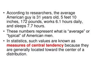
According to researchers, the average American guy is 31 years old, 5 feet 10 inches, 172 pounds, works 6.1 hours daily, and sleeps 7.7 hours. These numbers represent what is “average” or “typical” of American men.

E N D
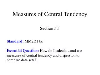
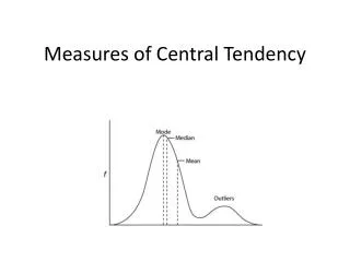
According to researchers, the average American guy is 31 years old, 5 feet 10 inches, 172 pounds, works 6.1 hours daily, and sleeps 7.7 hours. • These numbers represent what is “average” or “typical” of American men. • In statistics, such values are known as measures of central tendency because they are generally located toward the center of a distribution.
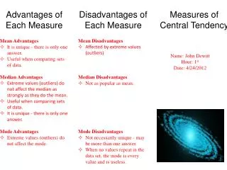
Measures of Central Tendency Mean Arithmetic average Sum of all data values divided by the number of data values in an array Most frequently used measure of central tendency Strongly influenced by outliers - very large or very small values
Measures of Central Tendency Determine the mean value of 48, 63, 62, 49, 58, 2, 63, 5, 60, 59, 55
Measures of Central Tendency Median • The middle number • Data values must be ordered from lowest to highest • If you have an odd number of data then the median is the value in the middle of the set • If you have an even number of data then the median is the average between the two middle values in the set • Useful in situations with skewed data and outliers
Measures of Central Tendency Determine the median value of 48, 63, 62, 49, 58, 2, 63, 5, 60, 59, 55 Organize the data array from lowest to highest value. 58, 59, 60, 62, 63, 63 2, 5, 48, 49, 55, Select the data value that splits the data set evenly. Median = 58 What if the data array had an even number of values? 60, 62, 63, 63 58, 59, 5, 48, 49, 55, Median = 58.5
Position of the Median • If n data items are arranged in order, from smallest to largest, the median is the value in the (n + 1) / 2 position
Measures of central tendency Mode • Most frequently occurring response within a data array • May not exist at all • If no numbers repeat then the mode = 0 • Bimodal & multimodal
Measures of Central Tendency Determine the mode of 48, 63, 62, 49, 58, 2, 63, 5, 60, 59, 55 Mode = 63 Determine the mode of 48, 63, 62, 59, 58, 2, 63, 5, 60, 59, 55 Mode = 63 & 59 Bimodal Determine the mode of 48, 63, 62, 59, 48, 2, 63, 5, 60, 59, 55 Mode = 63, 59, & 48 Multimodal
Suppose your six exam grades in a class are: • 52, 69, 75, 86, 86, 92. • Compute your final grade (90-100 = A, 80-89 = B, 70-79 = C, 60-69 = D, below 60 = F) using the: • a. mean b. median c. mode • d. Find the median position
Meaures of Dispersion Measure of data scatter Range Difference between the lowest and highest data value Standard Deviation Square root of the variance Variance Average of squared differences between each data value and the mean
Range Calculate by subtracting the lowest value from the highest value. Calculate the range for the data array. 2, 5, 48, 49, 55, 58, 59, 60, 62, 63, 63
Standard Deviation • Calculate the mean . • Subtract the mean from each value. • Square each difference. • Sum all squared differences. • Divide the summation by the number of values in the array minus 1. • Calculate the square root of the product.
Standard Deviation Calculate the standard deviation for the data array. 2, 5, 48, 49, 55, 58, 59, 60, 62, 63, 63 1. 2. 2 – 47.64 = -45.64 5 – 47.64 = -42.64 48 – 47.64 = 0.36 49 – 47.64 = 1.36 55 – 47.64 = 7.36 58 – 47.64 = 10.36 59 – 47.64 = 11.36 60 – 47.64 = 12.36 62 – 47.64 = 14.36 63 – 47.64 = 15.36 63 – 47.64 = 15.36
Standard Deviation Calculate the standard deviation for the data array. 2, 5, 48, 49, 55, 58, 59, 60, 62, 63, 63 3. 11.362 = 129.05 12.362 = 152.77 14.362 = 206.21 15.362 = 235.93 15.362 = 235.93 (-45.64)2 = 2083.01 (-42.64)2 = 1818.17 0.362 = 0.13 1.362 = 1.85 7.362 = 54.17 10.362 = 107.33
Standard Deviation Calculate the standard deviation for the data array. 2, 5, 48, 49, 55, 58, 59, 60, 62, 63, 63 4. 2083.01 + 1818.17 + 0.13 + 1.85 + 54.17 + 107.33 + 129.05 + 152.77 + 206.21 + 235.93 + 235.93 = 5,024.55 7. 5. 11-1 = 10 6. S = 22.42
Standard Deviation • The standard deviation measures the spread of the distribution or the dispersion the distribution has. • The larger the standard deviation, the more spread out the distribution is. • The smaller the standard deviation, the less spread the distribution has.
Variance • Steps 1 – 5 of the standard deviation: • Calculate the mean. • Subtract the mean from each value. • Square each difference. • Sum all squared differences. • Divide the summation by the number of values in the array minus 1.
Variance Calculate the variance for the data array. 2, 5, 48, 49, 55, 58, 59, 60, 62, 63, 63
Variance (s2) • Mathematically expressing the degree of variation of data from the mean • A large variance means that the individual data of the sample deviate a lot from the mean. • A small variance indicates the data deviate little from the mean