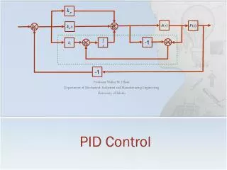
PD, PI, PID Compensation
PD, PI, PID Compensation. M. Sami Fadali Professor of Electrical Engineering University of Nevada. Outline. PD compensation. PI compensation. PID compensation. PD Control. L = loop gain = N / D . s cl = desired closed-loop pole location.


PD, PI, PID Compensation
E N D
Presentation Transcript
PD, PI, PID Compensation M. Sami Fadali Professor of Electrical Engineering University of Nevada
Outline • PD compensation. • PI compensation. • PID compensation.
PD Control • L= loop gain = N/ D. • scl = desired closed-loop pole location. • Find a controller C s.t. LC(scl)= 180 or its odd multiple (angle condition). • Controller Angle for scl Zero location
Remarks • Graphical procedures are no longer needed. • CAD procedure to obtain the design parameters for specified & n. » evalfr(l,scl) % Evaluate l at scl »polyval( num,scl) % Evaluate num at scl • The complex value and its angle can also be evaluated using any hand calculator.
Procedure:MATLAB or Calculator • Calculate L (scl) »theta = piangle(evalfr(l, scl) ) • Calculate zero location using (5.14). • Calculate new loop gain (with zero) » lc = tf( [1, a],1)*l • Calculate gain (magnitude condition) » K = 1/abs( evalfr( lc, scl)) 5. Check time response of PD-compensated system. Modify the design to meet the desired specifications if necessary (MATLAB).
Procedure 5.2: Given e() & • Obtain error constant Ke from e()and determine a system parameter Kfthat remains free after Ke is fixed for the system with PD control. 2- Rewrite the closed-loop characteristic equation of the PD controlled system as
Procedure 5.2 (Cont.) • Obtain Kf corresponding to the desired closed-loop pole location. As in Procedure 5.1, Kfcan be obtained by clicking on the MATLAB root locus plot or applying the magnitude condition using MATLAB or a calculator. • Calculate the free parameter from the gain Kf. • Check the time response of the PD compensated system and modify the design to meet the desired specifications if necessary.
Example 5.5 Use a CAD package to design a PD controller for the type I system to meet the following specifications (a) = 0.7 & n = 10 rad/s. (b) = 0.7 & e()=4% due to a unit ramp.
(a) =0.7 & n=10 rad/s MATLAB: calculate pole location & corresponding gain » scl = 10*exp( j*( pi-acos(0.7) ) ) scl = 7.0000 + 7.1414I » g=zpk([ ],[0,-4],1);theta=pi( angle( evalfr( g, scl) ) ) theta = 1.1731 » a = 10 * sqrt(1-0.7^2)/ tan(theta) + 7 a = 10.0000 » k =1/abs(evalfr(tf( [1, a],1)*l,scl)) % Gain at scl k = 10.0000
(b) =0.7, e()=4% for unit ramp Closed-loop characteristic equation with PD Assume that K varies with K a fixed, then RL= circle centered at the origin
RL of PD-compensated System K afixed
(b) Design Cont. Desired location: intersection of root locus with = 0.7 radial line. K = 10, a =10 (same values as in Example 5.3). MATLAB command to obtain the gain » k = 1/abs( evalfr( tf([1,10],[ 1, 4, 0]), scl) ) k = 10.0000 • Time responses of two designs are identical.
PI Control • Integral control to improve e(), (increases type by one) worse transient response or instability. • Add proportional control controller has a pole and a zero. • Transfer function of proportional-plus-integral (PI) controller
PI Remarks • Used in cascade compensation (integral term in the feedback path is equivalent to a differentiator in the forward path) • PI design for a plant transfer function G(s) = PD design of G(s)/ s. • A better design is often possible by "almost canceling" the controller zero and the controller pole (negligible effect on time response).
Procedure 5.3 • Design a proportional controller for the system to meet the transient response specifications, i.e. place the dominant closed-loop system poles at scl= zwnjwd . • Add a PI controller with the zero location (- a) = small angle ( 3 5). • Tune the gain of the system to move the closed-loop pole closer to scl.
Comments • Use PI control only if P-control meets the transient response but not the steady-state error specifications. Otherwise, use another control. • Use pole-zero diagram to prove zero location formula.
Proof Controller angle at scl From Figure
Proof (Cont.) Trig. identity Solve for x x = ( a/ n)Multiplying by n givesa.
Example 5.6 Design a controller for the position control system to perfectly track a ramp input with a dominant pair with = 0.7 & wn =4 rad/s.
Solution • Procedure 5.1 with modified transfer function. • Unstable for all gains (see root locus plot). • Controller must provide an angle 249 at the desired closed-loop pole location. • Zero at 1.732. • Cursor at desired pole location on compensated system RL gives a gain of about 40.6.
Analytical Design Closed-loop characteristic polynomial Values obtained earlier, approximately.
MATLAB » scl = 4*exp(j*(pi acos( 0.7)) ) scl = -2.8000 + 2.8566i » theta = pi + angle( polyval( [ 1, 10, 0, 0], scl ) ) theta = 1.9285 » a = 4*sqrt(1-.7^2)/tan(theta)+ 4*.7 a = 1.7323 » k = abs(polyval( [ 1, 10, 0,0], scl )/ polyval([1,a], scl) ) k = 40.6400
Design I Results Closed-loop transfer function for Design I Zero close to the closed-loop poles excessive PO (see step response together with the response for a later design: Design II).
Step Response of PI-compensated System Design I (dotted), Design II (solid).
Design II: Procedure 5.3 = 0.7, K 51.02 & n = 7.143 rad/s. (acceptable design) zero location Closed-loop transfer function Gain slightly reduced to improve response. Dominant poles 0.7,n= 6.6875 rad/s Time response for Designs I and II PO for Design II (almost pole-zero cancellation) << Design I (II better)
PID (proportional-plus-integral-plus-derivative) Control • Improves both transient & steady-state response. • Kp, Ki , Kd= proportional, integral, derivative gain, resp. • Controller zeros: real or complex conjugate.
PID Design Procedures • Cancel real or complex conjugate LHP poles. • Cancel pole closest to (not on) the imaginary axis then add a PD controller by applying Procedures 5.1 or 5.2 to the reduced transfer function with an added pole at the origin. • Follow Procedure 5.3 with the proportional control design step modified to PD design. The PD design meets the transient response specifications and PI control is then added to improve the steady-state response.
Example 5.7 Design a PID controller for the transfer function to obtain zero e() due to ramp, = 0.7 and n = 4 rad/s.
Design I Cancel pole at 1 with a zero & add an integrator Same as transfer function of Example 5.6 Add PD control of 5.6 PID controller
Design II Design PD control to meet transient response specs. Select n = 5 rad/s (anticipating effect of adding PI control). Design PD controller using MATLAB commands » [k,a,scl] = pdcon(0.7, 5, tf(1, [1,11,10,0]) ) k = 43.0000 a = 2.3256 scl = -3.5000 + 3.5707i » b =5 /(0.7 + sqrt(1-.49)/tan(3*pi/ 180) ) % Obtain PI zero. b = 0.3490 Transfer function for Design II (reduce gain to 40 to correct for PI)
Conclusions • Compare step responses for Designs I and II: Design I is superior because the zeros in Design II result in excessive overshoot. • Plant transfer function favors pole cancellation in this case because the remaining real axis pole is far in the LHP. If the remaining pole is at 3, say, the second design procedure would give better results. • MORAL: No easy solutions in design, only recipes to experiment with until satisfactory results are obtained.
Example 5.8 Design a PID controller for the transfer function to obtain zero e()due to step, = 0.7 and n 4 rad/s
Solution • Complex conjugate pair slows down the time response. • Third pole is far in the LHP. • Cancel the complex conjugate poles with zeros and add an integrator
Solution (cont.) • Stable for all gains. • Closed-loop characteristic polynomial Equate coefficients with = 0.7 (meets design specs.) PID controller
Step Response of PID-compensated System In practice, pole-zero cancellation may not occur but near cancellation is sufficient to obtain a satisfactory time response