Download
1 / 29
290 likes | 573 Vues
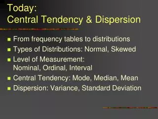
Today: Central Tendency & Dispersion. From frequency tables to distributions Types of Distributions: Normal, Skewed Level of Measurement: Nominal, Ordinal, Interval Central Tendency: Mode, Median, Mean Dispersion: Variance, Standard Deviation.

E N D
Today:Central Tendency & Dispersion • From frequency tables to distributions • Types of Distributions: Normal, Skewed • Level of Measurement: Nominal, Ordinal, Interval • Central Tendency: Mode, Median, Mean • Dispersion: Variance, Standard Deviation
Descriptive statistics are concerned with describing the characteristics of frequency distributions • Where is the center? • What is the range? • What is the shape [of the distribution]?
Range • Difference of the greatest value and the smallest value • Ex. 1290, 1310, 1420, 1450, 1460, 1900, 1900, 1980, 2540
Frequency TableTest Scores Find the Range Score Frequency 65 1 70 2 75 3 80 4 85 3 90 2 95 1
Frequency Distributions 4 3 2 1 Frequency 65 70 75 80 85 90 95 Test Score
Summarizing Distributions Two key characteristics of a frequency distribution are especially important when summarizing data or when making a prediction from one set of results to another: • Central Tendency • What is in the “Middle”? --Median • What is most common? --Mode • What would we use to predict? • Dispersion • How Spread out is the distribution? --Range • What Shape is it?
Three measures of central tendencyare commonly used in statistical analysis - the mode, the median, and the mean Each measure is designed to represent a typical score The choice of which measure to use depends on: • the shape of the distribution (whether normal or skewed), and
Mode • Most Common Outcome Ex. 1290, 1310, 1420, 1450, 1460, 1900, 1900, 1980, 2540 Male Female
Median • Middle-most Value • 50% of observations are above the Median, 50% are below it • Therefore, it is not sensitive to outliers • Formula Median = n + 1 / 2
To compute the median · first you rank order the values of X from low to high: 85, 94, 94, 96, 96, 96, 96, 97, 97, 98 · then count number of observations = 10. · add 1 = 11. · divide by 2 to get the middle score the 5½ score here 96 is the middle score score
Median • Find the Median 4 5 6 6 7 8 9 10 12 • Find the Median 5 6 6 7 8 9 10 12 • Find the Median 5 6 6 7 8 9 10 100,000
Mean - Average • Most common measure of central tendency • Best for making predictions
Finding the Mean • X = Sum of the numbers divided by the total number of numbers • If X = {3, 5, 10, 4, 3} X = (3 + 5 + 10 + 4 + 3) / 5 = 25 / 5 = 5
Find the Mean & Median Q: 4, 5, 8, 7 A: 6 Median: 6 Q: 4, 5, 8, 1000 A: 254.25 Median: 6.5
IF THE DISTRIBUTION IS NORMAL Mean is the best measure of central tendency Most scores “bunched up” in middle Extreme scores less frequent don’t move mean around.
Measures of Variability Central Tendency doesn’t tell us everything Dispersion/Deviation/Spread tells us a lot about how a variable is distributed.
Dispersion Once you determine that the variable of interest is normally distributed, ideally by producing a histogram of the scores, the next question to be asked about the data is its dispersion: how spread out are thescores around the mean. Dispersion is a key concept in statistical thinking. The basic question being asked is how much do the scores deviate around the Mean? The more “bunched up” around the mean the better your ability to make accurate predictions.
Means • Consider these means for weekly candy bar consumption. X = {7, 8, 6, 7, 7, 6, 8, 7} X = (7+8+6+7+7+6+8+7)/8 X = 7 X = {12, 2, 0, 14, 10, 9, 5, 4} X = (12+2+0+14+10+9+5+4)/8 X = 7 What is the difference?
What if scores are widely distributed? The mean is still your best measure and your best predictor, but your predictive power would be less.
Mean Absolute Deviation The key concept for describing normal distributions and making predictions from them is called deviation from the mean. We could just calculate the average distance between each observation and the mean. • We must take the absolute value of the distance, otherwise they would just cancel out to zero! Formula:
Mean Absolute Deviation: An Example Data: X = {6, 10, 5, 4, 9, 8} X = 42 / 6 = 7 • Compute X (Average) • Compute X – X and take the Absolute Value to get Absolute Deviations • Sum the Absolute Deviations • Divide the sum of the absolute deviations by N 12 / 6 = 2 Total: 12
What Does it Mean? • On Average, each observation is two units away from the mean. Is it Really that Easy? • No! • Absolute values are difficult to manipulate algebraically
Mode: Range: Median Example: Mean: Data: X = {6, 10, 5, 4, 9, 8} Mean Absolute Deviation: