Encoding and Image Formation
Encoding and Image Formation. Gradients Slice selection Frequency encoding Phase encoding Sampling Data collection. Introduction. Encoding means the location of the MR signal and positioning it on the correct place in the image

Encoding and Image Formation
E N D
Presentation Transcript
Encoding and Image Formation Gradients Slice selection Frequency encoding Phase encoding Sampling Data collection
Introduction • Encoding means the location of the MR signal and positioning it on the correct place in the image • RF at precessional frequency of hydrogen applied at 900 to B0 resonates and flips the NMV into transverse plane. • The individual magnetic moments of hydrogen is put into phase. • The coherent transverse magnetization precesses at Larmor frequency in the transverse plane.
A voltage (signal) is induced in the receiver coil placed in the transverse plane • This signal has a frequency equal to Larmor frequency of hydrogen (at 1.5 T : 63.86 MHz) • The system must be able to locate the signal spatially in three dimensions, so that it can position each signal at the correct point on the image. • First it locates a slice. • Then it is located or encoded along both axes of the image. • This task is performed by magnetic gradients
Magnetic Gradients • Gradients are alterations to the main magnetic field and are generated by coils of wire located within the bore of the magnet. • The passage of current through a gradient coil induces a gradient magnetic field. • The gradient field either adds to or subtracts from B0. • B0 is altered in a linear fashion.
Magnetic field strength and therefore the precessional frequency of the nuclei situated in the long axis is deferent and is predictable. • This is called spatial encoding positive gradient 1 G per cm negative A B C 2 cm 2 cm 9998 G 42.5614 MHz 10002 G 42.5785 MHz 10000 G 42.57 MHz
There are three gradient coils (X,Y,Z) situated within the bore of the magnet • Z gradient alters the magnetic field strength along the Z- (long) axis • Y gradient alters the magnetic field strength along the Y- (vertical) axis of the magnet • X gradient alters the magnetic field strength along the X- (horizontal /transverse) axis of the magnet Y Z X
The magnetic isocentre is the centre point of the axis of all three gradients, and the bore of the magnet. • The field strength remains unaltered at the isocentre isocentre Y Z X
Steep & shallow gradients • When a gradient coil is switched on, the magnetic field strength is either subtracted from or added to B0 relative to the isocentre • The slope of the resulting magnetic field is the amplitude of the magnetic field gradient and it determines the rate of change of the magnetic field strength along the gradient axis. • Steep gradient slopes alter the magnetic field strength between two points more than shallow gradient slopes. • Steep gradient slopes therefore alter the precessional frequency of nuclei between two points, more than shallow gradients slopes
Slice selection • This is done by • first switching the appropriate gradient coil to alter the field strength and the precessional frequency at points along the corresponding axis, and • then by transmitting a selected band of RF frequencies to selectively excite the nuclei which precess in that particular frequencies. • Resonance of nuclei within the slice occurs because RF appropriate to that position is transmitted • Nuclei situated in other slices does not resonate because their precessional frequency is different.
Z-gradient selects axial slices • Y gradient selects coronal slices • X gradient selects sagittal slices Y Z X
Slice thickness • To give each slice a thickness, a band of nuclei must be excited by the excitation pulse • The slope of the slice-select gradient determines the difference in precessional frequency between two points on the gradient. • Once a certain gradient slope is applied, the RF pulse transmitted to excite the slice, must contain a range of frequencies to match the difference in precessional frequency between two points • This frequency range is called the bandwidth. • As the RF is being transmitted at this point it is called the transmit bandwidth.
To achieve thin slices, a steep slice select slope and/or narrow bandwidth is applied • To achieve thick slices, a shallow slice select slope and/or broad transmit bandwidth is applied. Steep gradient Shallow gradient slice select gradient broad Bandwidth Transmit bandwidth Narrow Bandwidth Thick slice Thin slice Thin slice Thick slice
Gradient strength & slice thickness Shallow (weaker gradient) Steeper ( strong) gradient
In Practice • The system automatically applies the appropriate gradient slope and transmitbandwidth according to the thickness of slice required. • The slice is excited by transmitting RF at the centre frequency corresponding to the precessional frequency of nuclei in the middle of the slice, • The bandwidth and gradient slope determine the range of nuclei that resonate on either side of the centre.
The gap between the slices is determined by the gradient slope and by the thickness of the slice. • In spin echo pulse sequences, the slice select gradient is switched on during the application of the 900 excitation pulse and during the 1800 rephasing pulse, to excite and rephase each slice selectively. • In gradient echo, the slice select gradient is switched on during the excitation pulse only. 1800 900 900 Slice select gradient
Frequency encoding • Once a slice has been selected, the signal coming from it must be spatially located (encoded) along both axes of the image • Locating the signal along the long axis of anatomy is done by a process called frequency encoding • A gradientis applied along theselected axis • The precessional frequency of signal along the axis is therefore altered in a linear fashion. • The signal can now be located along the axis of the gradient according to its frequency
A B C For frequency encoding of • Coronal & sagittal images – use z gradient • Axial images – use X gradient • Axial images of Head – use Y gradient Nuclei in column A precess at frequency A Nuclei in column C precess at frequency C Nuclei in column B precess at frequency B
In practice • The frequency encoding gradient is switched on when the signal is received and is often called the readout gradient 1800 900 900 FID Echo FID rephasing dephasing Frequency encoding gradient peak The steepness of the slope of the frequency encoding gradient determines the size of the anatomy covered ; Field Of View (FOV) along the axis during scan.
Phase encoding • The location of the signal along the remaining third axis is achieved by a process called phase encoding. • This is achieved by applying a gradient along this remaining axis • A gradient is switched on it alters the speed of precession as well as the accumulated phase of the nuclei along their precessional path. • It produces a phase difference or shift betweennuclei positioned along the axis.
Gradient & phase difference nuclei travel slower 14998 G 63.852 MHz Loose phase 15000 G 63.86 MHz Nuclei travel faster 15002 G 63.868 MHz gain phase
When the phase encoding gradient is switched off, the magnetic field strength experienced by the nuclei returns to B0 and the precessional frequency of all the nuclei returns to the larmor frequency. • However the phase difference between nuclei remains • The nuclei travel at the same speed around their precessional paths, but their phases or positions are different. • This difference in phase between the nuclei is used to determine their position along the phase encoding gradient (axis).
In practice • The phase encoding gradient is switched on just before the application of the 1800 rephasing pulse in spin echo sequences. 1800 900 900 Phase encoding gradient
Summary of phase encoding • The phase encoding gradient alters the phase along the short axis of the anatomy • In Coronal images – x gradient • In sagittal images - Y gradient • In axial images - Y gradient • Axial images of brain – x gradient
Summary spatial encoding • The slice-select gradient is switched on • during the 90 and 180 pulses in spin echo pulse sequences , and • during the excitation pulse only in gradient echo pulse sequences • The slope of the slice-select gradient determines the slice thickness and slice gap (along with transmit bandwidth)
The phase encoding gradient is switched on • just before the 180 pulse in spin echo, and • between excitation and the signal collection in gradient echo. • The slope of the phase encoding gradient determines the degree of phase shift along the phase encoding axis. • The frequency encoding gradient is switched on during the collection of the signal • The amplitude of the frequency encoding gradient and the phase encoding gradient determines the two dimensions of the FOV
Gradient timing in spin echo TR 1800 900 900 echo Phase encode slice select slice select Frequency encode
Sampling • The signal is collected during the frequency encoding gradient (readout gradient) • The duration of readout gradient is called sampling time • The system samples up to 1024 frequencies during sampling time • The rate at which the samples are taken is called the sampling rate
The number of samples taken determines the number of frequencies sampled • The range of frequencies is called the receive bandwidth Frequency columns in FOV f1 f2 f3 f4 f5 f6 Frequencies sampled are mapped across the FOV along the frequency axis Receive bandwidth
Sampling time, sampling rate and receive bandwidth are linked by a mathematical principle called the Nyquist theorem. • It states that any signal must be sampled at least twice per cycle in order to represent or reproduced it acurately. • In addition enough cycles must occur during the sampling time to achieve enough frequency samples ( if 256 samples are to be taken 128 cycles must occur during the sampling time) • Number of cycles occurring per second is determined by the receive bandwidth • Receive bandwidth is proportional to the Sampling rate
Sampling time is inversely proportional to: • The sampling rate • The receive bandwidth The receive bandwidth affect the minimum TE ( because the sampling time is changed) • Reducing the receive bandwidth increase the TE (sampling time increases) & vise versa • Usually the receive bandwidth & sampling time are fixed
Nyquist theorum Sampling once Reproduced as a straight line Sampling twice Reproduced more accurately
Bandwidth versus sampling time Sampling time (8 ms) Bandwidth 128 cycles occur (256 samples can be taken) 16,000 Hz 64 cycles occur (only 128 samples can be taken) 8,000 Hz If bandwidth is reduced, the sampling time must be increased so that the same number of samples can be taken
Data collection • Location of individual signals within the image by measuring the number of times the magnetic moments cross the receiver coil (frequency), and their position around their precessional path (phase) Frequency shift 3 cycles/s 2 cycles/s 1 cycle/s Phase shift
K space • The data information is stored in the computer memory location called the K space. Maximum number of lines are 1024 frequency +ve outer One line is filled for one phase encoding gradient central phase -ve
Data collection – step 1 • During each TR the signal from each slice is phase encoded and frequency encoded. • A certain value of frequency shift is obtained according to the slope of the frequency encoding gradient, which is determined by the size of the FOV. • As the FOV remains unchanged during the scan, the frequency shift value remains the same. • A certain value of phase shift is also obtained according to the slope of the phase encoding gradient • The slope of the phase encoding gradient will determine which line of K space is filled with the data from that frequency and phase encoding
Phase shift & pseudo-frequency • The system cannot measure the phase values directly • It can measure frequency • The phase shift values are converted to a sine wave • The frequency of this sine wave is called a pseudo-frequency • Different phase shift gradient produce different sine waves with different pseudo-frequency
The pseudo frequency curve time Phase shift value
Phase encoding gradient & pseudo frequency • Steeper gradients results in high pseudo frequencies • Shallow gradients results in low frequencies
In order to fill out different lines of K space, the slope of the phase encoding gradient must be altered after each TR • With each phase encoding one line of Kspace is filled • Different lines in K space are filled after every TR • The phase encoding gradient is altered for every TR • In order to complete the acquisition all the lines of selected K space must have been filled • The number of lines that are filled is determined by the number of different phase encoding slopes that are applied
Fast Fourier Transform (FFT) • The data in K space is converted into an image mathematically by Fourier Transform. • The receive signal is a composite of multiple signals with different frequencies and amplitudes • The signal intensity/time domain is converted to a signal intensity/frequency domain Amplitude RF intensity Frequency Time Frequency domain Time domain
Matrix & FOV • The FOV relates to the amount of anatomy covered • It can be square or rectangular • Image consists of a matrix of pixels • Te number of pixels depends on the number of frequency samples and phase encodings • Matrix = frequency samples x phase encodings
Matrix 4 frequency samples 8 frequency samples 4 phase samples 8 phase samples Coarse matrix 4x4 Fine matrix 8 x 8
Data collection - step 2, NSA (NEX) • When all the lines of K space is filled the acquisition is over • But the signal can be sampled more than once with the same slope of phase encoding gradient. • Doing so each line of K space is filled more than once • The number of times each signal is sampled with the same slope of phase encoding gradient is usually called the number of signal averages (NSA) or the number of excitations (NEX). • The higher the NEX, the more data is stored and the amplitude of the signal at each frequency and phase shift is greater
Scan timing • Every TR, each slice is selected, phase encoded and frequency encoded. • The maximum number of slices that can be selected and encoded depends on the length of the TR. • E.g. • TR of 500ms may allow 12 slices. • TR of 2000 ms may allow 18 slices
TR & number of slices 180 TR 90 echo Slice 1 TE Slice 2 Slice 3 Phase encode 1 Slice 4 Slice 1 second TR Phase encode 2
The phase encoding gradient slope is altered every TR and is applied to each selected slice in order to phase encode it. • At each phase encode a different line of k space is filled. The number of phase encoding steps therefore affects the length of the scan • E.g. 256 phase encodings require 256 x TR to complete the scan. • The scan time is also affected by the number of times the signal is phase encoded with the same phase encoding gradient slope, or NEX . So, Scan time = TR x Number of phase encodings x NEX
K space filling • The negative half of the k space is a mirror image of the positive half. • The polarity of the phase gradient determines whether the positive or negative half is filled • Gradient polarity depends on the direction of the current through the gradient coil • The central lines are filled with data produced after the application of shallow phase encoding gradients • The outer lines are filled with data produced with steep phase encoding gradients
The steepness of the slope of the phase encoding gradient depends on the current driven through he coil. • The central lines of K space are usually filled first. (if 256 phase encodings are performed 128 positive lines and 128 negative lines are filled. • The lines are usually filled sequentially either from top to bottom or from bottom to top