GIS Technology in Transition Moving Maps to Mapped Data, Spatial Analysis and Beyond

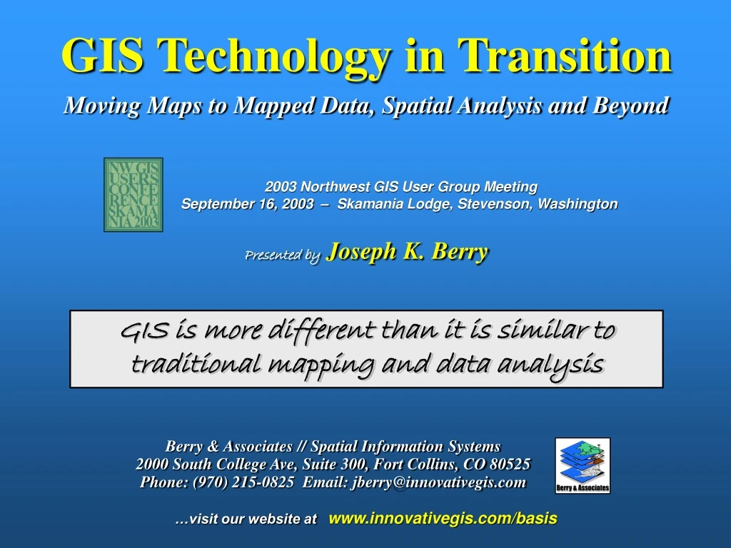
2003 Northwest GIS User Group Meeting September 16, 2003 – Skamania Lodge, Stevenson, Washington Berry & Associates // Spatial Information Systems2000 South College Ave, Suite 300, Fort Collins, CO 80525Phone: (970) 215-0825 Email: jberry@innovativegis.com GIS Technology in TransitionMoving Maps to Mapped Data, Spatial Analysis and Beyond Presented byJoseph K. Berry GIS is more different than it is similar to traditional mapping and data analysis …visit our website atwww.innovativegis.com/basis

Traditional Mapping manually drafted map Computer Mapping automates the cartographic process (70s) Spatial Database Management links computer mapping techniques with traditional database capabilities (80s) GIS Modeling representation of relationships within and among mapped data (90s) Historical Setting and GIS Evolution (Berry)

WHERE – Digital Map Mapped data can be queried by interacting with the map (where) or database (what) 1)Select forest type Aspen, SP1= Aw 2) Select tall Aspen stands, Height > 20m WHAT -- database Query Builder Map Display Connectivity and Map Delivery SDT, www.spatialdatatech.com Indelix, www.idelix.com Where is What …and Wow (Berry)

WHERE IS WHAT Vector-based processing provides Mapping and Geo-Query capabilities that repackage existing spatial data as reports and displays WHY AND SO WHAT Discrete Objects Descriptive Mapping Grid-based processing provides Map Analysis capabilities that derive new information on relationships within and among mapped data Continuous Surfaces Prescriptive Mapping Where is What and Wow to…Why and So What (Berry)

Script Logic Simple Erosion Model …GIS Modeling involves logical sequencing of map analysis operations …a Command Macro Language consists of a graphical interface for entering, editing, executing, documenting, storing and retrieving a GIS Model (Berry)

Effectively far away, though right near a stream …how can that be? …what about different soils? …what about roughness? …or time of year? Variable-Width Buffer(Sediment loading) Simple Buffer (Berry)

Characterizing Surface Flow The relative amount of water passing through each grid cell is determined by simulating a drop of water landing in each cell and proceeding downhill by the steepest path. The number of paths crossing each location identifies the total uphill confluence. Micro Terrain Analysis Calculation of slope considers the arrangement and magnitude of elevation differences “Map-ematics” Characterizing Slope (and Aspect) A digital terrain surface is formed by assigning an elevation value to each cell in an analysis grid. The “slant” of the terrain at any location can be calculated– inclination of a plane fitted to the elevation values of the immediate vicinity. (See Map Analysis, “Topic 11” for more information) (Berry)

Map Analysis • Surface Modelingmaps the spatial distribution and pattern of point data… • Map Generalization— characterizes spatial trends (e.g., titled plane) • Spatial Interpolation— deriving spatial distributions (e.g., IDW, Krig) • Other— roving window/facets (e.g., density surface; tessellation) • Data Mininginvestigates the “numerical” relationships in mapped data… • Descriptive— aggregate statistics (e.g., average/stdev, similarity, clustering) • Predictive— relationships among maps (e.g., regression) • Prescriptive— appropriate actions (e.g., optimization) • Spatial Analysisinvestigates the “contextual” relationships in mapped data… • Reclassify— reassigning map values (position; value; size, shape; contiguity) • Overlay— map overlay (point-by-point; region-wide; map-wide) • Distance— proximity and connectivity (movement; optimal paths; visibility) • Neighbors— ”roving windows” (slope/aspect; diversity; anomaly) (Berry)

Spatial Interpolation(Geographic Distribution) “Surface Modeling” is similar to slapping a big chunk of modeler’s clay over the “data spikes,” then taking a knife and cutting away the excess to leave a continuous surface that encapsulates the peaks and valleys implied by the spatial pattern of the field samples …nearby things are more alike than distant things (Berry)

Non-Spatial statistics seeks the “typical” condition and applies uniformly throughout geographic space-- AVERAGE Spatial Statistics seeks to map the variance Spatial Interpolation is similar to throwing a blanket over the “data spikes” to conforming to the geographic pattern of the data. Mapping the Variance (Berry)

What spatial relationships do you see? Visualizing Spatial Relationships Interpolated Spatial Distribution Phosphorous (P) …do relatively high levels of P often occur with high levels of K and N? …how often? …where? (Berry)

Clustering Maps …groups of “floating balls” in data space identify locations in the field with similar data patterns– data zones (Berry)

The Precision Ag Process(Fertility example) Steps 1) – 3) Step 5) Prescription Map On-the-Fly Yield Map Map Analysis Step 4) Cyber-Farmer, Circa 1992 Farm dB Zone 3 Zone 2 Variable Rate Application Zone 1 Step 6) As a combine moves through a field 1) it uses GPS to check its location then 2) checks the yield at that location to 3) create a continuous map of the yield variation every few feet. This map 4) is combined with soil, terrain and other maps to derive a 5) “Prescription Map” that is used to 6) adjust fertilization levels every few feet in the field. (Berry)

Mapped data that exhibits high spatial dependency create strong prediction functions. As in traditional statistical analysis, spatial relationships can be used to predict outcomes …the difference is that spatial statistics predicts where responses will be high or low Spatial Data Mining …making sense out of a map stack (Berry)

Precision Conservation Wind Erosion Chemicals Soil Erosion Runoff Leaching Leaching Leaching 3-dimensional SPATIAL ANALYSIS 2-dimensional Interconnected Perspective Isolated Perspective Precision Ag to Precision Conservation From a Field perspective to Watershed, Landscape and Ecosystem perspective Precision Ag SURFACE MODELING SPATIAL DATA MINING (Berry)

1) Pipeline X 2) Spill Point #1 X 5) Flowing Water 3) HCA 4) Report HCA Impact 1) The Pipeline is positioned on the Elevation surface 2) Flow from Spill Points along the pipeline are simulated 3)High Consequence Areas (HCA) are identified 4) A Report is written identifying flow paths that cross HCA areas 5) Overland flow is halted when Flowing Water is encountered (Channel Flow Model) Spill Migration Modeling Overland Flow Model Elevation Surface (Berry)

Types of Surface Flows Common sense suggests that “water flows downhill” however the corollary is “…but not always the same way.” (Berry)

Characterizing Overland Flow and Quantity Intervening terrain and conditions form Flow Impedance and Quantity maps that are used to estimate flow time and retention (Berry)

Simulating Different Product Types Physical properties combine with terrain/conditions to model the flow of different product types Flow Velocity is a function of— Specific Gravity (p), Viscosity (n) and Depth (h) of product Slope Angle (spatial variable computed for each grid cell) (Berry)

The minimum time for flows from all spills… characterizes the impact for the High Consequence Areas Flows from spill 1, 2 and 3 Impacted portion of the Drinking water HCA Drinking water HCA Characterizing Impacted Areas (Berry)

3)Impacted HCA Times HCA Base Point 4)Report of Impacted HCA’s Out= 9.86 hr 0 hr HCA In= 11.46 hr HCA HCA X = 12.10 + .36 = 12.46 hr away from Base Point 7.3 hr HCA 13.6 hr X 9.6 hr 11.2 hr 2) Overland Flow Entry Time 8.4 hr HCA Overland Flow (2.5 hours) 13.1 hr 11.2 hr .12 1) Channel Flow Time .12 .14 13.1 hr 10.1 hr .27 X 2.5 + (12.46 -11.46) = 3.5 hours total 10.8 hr .25 .72 .78 1)Channel Flow times along stream network segments are added 2)Overland Flow time and quantity at entry is noted 3)Impacted High Consequence Areas (HCA) are identified 4)Report is written identifying flow paths that cross HCA areas Modeling Stream Channel Flow Channel Flow Model (Berry)

…customer flow along a road network is similar to water flowing in a stream channel …a Travel-time Map identifies the time to travel from anywhere to a store Modeling Customer Flow (Berry)

… travel-time surfaces for two different stores … can be compared for relative travel-time advantage Competition Analysis (Berry)

Existing Powerline Goal– identify thebest route for an electric transmission linethat considers various criteria for minimizing adverse impacts. Proposed Substation Houses • Criteria – the transmission line route should… • Avoid areas ofhigh housing density • Avoid areas that arefar from roads • Avoid areaswithin or near sensitive areas • Avoid areas of highvisual exposure to houses Roads Sensitive Areas Elevation Houses Transmission Line Siting Model (Berry)

PROPOSED SUBSTATION (END) EXISTING POWERLINE (START) ELEVATION MOST PREFERRED ROUTE ACCUMULATED COST SURFACE Step 3.The steepest downhill path from the Substation over the Accumulated Cost surface identifies the “least cost path”— Most Preferred Route avoiding areas of high visual exposure HOUSES VISUAL EXPOSURE TO HOUSES DISCRETE COST MAP Step 2.Accumulated Cost from the existing powerline to all other locations is generated based on the Discrete Cost map. Step 1.Visual Exposure levels (0-40 times seen) are translated into values indicating relative cost (1=low to 9=high) for siting a transmission line at every location in the project area. Routing and Optimal Paths AVOID AREAS OF HIGH VISUAL EXPOSURE TO HOUSES (Berry)

Considering Multiple Criteria Step 3Discrete Cost AVOID AREAS OF HIGH HOUSING DENSITY END HOUSING HOUSING DENSITY AVOID AREAS OF HIGH HOUSING DENSITY ENDING LOCATION BEST_ROUTE START STARTING LOCATION MOST PREFERRED ROUTE AVOID AREAS THAT ARE FAR FROM ROADS ACUMM_COST ROADS PROXIMITY TO ROADS AVOID AREAS THAT ARE FAR FROM ROADS ACCUMULATION SURFACE AVG_COST Step 3 Steepest Path AVERAGE COST AVOID AREAS IN OR NEAR SENSITIVE AREAS Step 2 Accumulated Cost SENSITIVE AREAS PROXIMITY TO SENSITIVE AREAS AVOID AREAS IN OR NEAR SENSITIVE AREAS • Criteria– the transmission line route should avoid… • Areas ofhigh housing density • Areas that arefar from roads • Areas within or near sensitive areas • Areas of highvisual exposure to houses AVOID AREAS OF HIGH VISUAL EXPOSURE ELEVATION VISUAL EXPOSURE TO HOUSES AVOID AREAS OF HIGH VISUAL EXPOSURE HOUSING Base Maps Derived Maps Cost/Avoidance Maps (Berry)

Considering Multiple Criteria Step 3Steepest Path AVOID AREAS OF HIGH HOUSING DENSITY END BEST_ROUTE START AVOID AREAS THAT ARE FAR FROM ROADS ACUMM_COST AVG_COST Step 3 Steepest Path AVOID AREAS IN OR NEAR SENSITIVE AREAS Step 2 Accumulated Cost • Criteria– the transmission line route should avoid… • Areas ofhigh housing density • Areas that arefar from roads • Areas within or near sensitive areas • Areas of highvisual exposure to houses AVOID AREAS OF HIGH VISUAL EXPOSURE Base Maps Derived Maps Cost/Avoidance Maps (Berry)

Step 1 Discrete Preference Map Least Most Preferred …average of the four individual preference maps … identifies the relative preference of locating a transmission line at any location throughout a project area considering multiple criteria (Berry)

Step 2 Accumulated Preference Map Splash Algorithm– like tossing a stick into a pond with waves emanating out and accumulating costs as the wave front moves … identifies the preference to construct the preferred transmission line from a starting location to everywhere in a project area (Berry)

Step 3 Most Preferred Route Preferred Route … the steepest downhill path over the accumulated preference surface identifies the most preferred route — minimizes areas to avoid (Berry)

Rankings Weights …but what is high housing density and how important is it? …etc? Model logic is captured in a flowchart where the boxes represent maps and lines identify processing steps leading to a spatial solution Siting Model Flowchart(Model Logic) Avoid areas of… High Housing Density Far from Roads In or Near Sensitive Areas High Visual Exposure (Berry)

1 for 0 to 5 houses …group consensus is that low housing density is most preferred Model calibration refers to establishing a consistent scale from 1 (most preferred) to 9 (least preferred) for rating each map layer Calibrating Map Layers(Relative Preferences) The Delphi Processis used to achieve consensus among group participants. It is a structured method involving iterative use of anonymous questionnaires and controlled feedback with statistical aggregation of group response. (Berry)

…group consensus is that housing density is very important (10.38 times more important than sensitive areas) HD * 10.38 R * 3.23 SA * 1.00 VE * 10.64 The Analytical Hierarchy Process (AHP)establishes relative importance among by mathematically summarizing paired comparisons of map layers’ importance. Model weighting establishes the relative importance among map layers (model criteria) on a multiplicative scale Weighting Map Layers(Relative Importance) (Berry)

The model is run using three different sets of weights for the map layers— …to generate three alternative routes (draped over Elevation) Generating Alternate Routes(changing weights) (Berry)

Where is What and Wow mapping, geo-query, delivery and display… Surface Modeling maps the spatial distribution and pattern of point data… Data Mining investigates the “numerical” relationships in mapped data… Spatial Analysis investigates the “contextual” relationships in mapped data… Transitioning Beyond Mapping (Berry)

…we’ve covered a lot, any questions? …for more importation online, see GIS Technology in Transition GIS technology is transitioning from Whereis What and Wow …to Whyand So What (Berry)

GIS Technology in Transition Moving Maps to Mapped Data, Spatial Analysis and Beyond