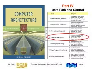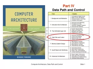
Part IV Data Path and Control
Part IV Data Path and Control. Try to achieve CPI = 1 with clock that is as high as that for CPI > 1 designs; is CPI < 1 feasible? (Chap 15-16). Design hardware for CPI = 1; seek improvements with CPI > 1 (Chap 13-14). Define an instruction set; make it simple enough

Part IV Data Path and Control
E N D
Presentation Transcript
Part IVData Path and Control Computer Architecture, Data Path and Control
Try to achieve CPI = 1 with clock that is as high as that for CPI > 1 designs; is CPI < 1 feasible? (Chap 15-16) Design hardware for CPI = 1; seek improvements with CPI>1 (Chap 13-14) Define an instruction set; make it simple enough to require a small number of cycles and allow high clock rate, but not so simple that we need many instructions, even for very simple tasks (Chap 5-8) A Few Words About Where We Are Headed Performance = 1 / Execution time simplified to1 / CPU execution time CPU execution time = Instructions CPI / (Clock rate) Performance = Clock rate / ( Instructions CPI ) Design memory & I/O structures to support ultrahigh-speed CPUs (chap 17-24) Design ALU for arithmetic & logic ops (Chap 9-12) Computer Architecture, Data Path and Control
IV Data Path and Control • Design a simple computer (MicroMIPS) to learn about: • Data path – part of the CPU where data signals flow • Control unit – guides data signals through data path • Pipelining – a way of achieving greater performance Computer Architecture, Data Path and Control
13 Instruction Execution Steps • A simple computer executes instructions one at a time • Fetches an instruction from the loc pointed to by PC • Interprets and executes the instruction, then repeats Computer Architecture, Data Path and Control
13.1 A Small Set of Instructions Fig. 13.1 MicroMIPS instruction formats and naming of the various fields. We will refer to this diagram later Seven R-format ALU instructions (add, sub, slt, and, or, xor, nor) Six I-format ALU instructions (lui, addi, slti, andi, ori, xori) Two I-format memory access instructions (lw, sw) Three I-format conditional branch instructions (bltz, beq, bne) Four unconditional jump instructions (j, jr, jal, syscall) Computer Architecture, Data Path and Control
op 15 0 0 0 8 10 0 0 0 0 12 13 14 35 43 2 0 1 4 5 3 0 fn 32 34 42 36 37 38 39 8 12 Copy The MicroMIPS Instruction Set Arithmetic Logic Memory access Control transfer Table 13.1 Computer Architecture, Data Path and Control
beq,bne 13.2 The Instruction Execution Unit syscall bltz,jr j,jal 22 instructions 12 A/L, lui, lw,sw Fig. 13.2 Abstract view of the instruction execution unit for MicroMIPS. For naming of instruction fields, see Fig. 13.1. Computer Architecture, Data Path and Control
13.3 A Single-Cycle Data Path Register writeback Instruction fetch Reg access / decode ALU operation Data access Fig. 13.3 Key elements of the single-cycle MicroMIPS data path. Computer Architecture, Data Path and Control
lui imm An ALU for MicroMIPS Fig. 10.19 A multifunction ALU with 8 control signals (2 for function class, 1 arithmetic, 3 shift, 2 logic) specifying the operation. Computer Architecture, Data Path and Control
13.4 Branching and Jumping (PC)31:2 + 1 Default option (PC)31:2 + 1 + imm When instruction is branch and condition is met (PC)31:28 | jta When instruction is j or jal (rs)31:2 When the instruction is jr SysCallAddr Start address of an operating system routine Update options for PC Lowest 2 bits of PC always 00 4 MSBs Fig. 13.4 Next-address logic for MicroMIPS (see top part of Fig. 13.3). Computer Architecture, Data Path and Control
13.5 Deriving the Control Signals Table 13.2 Control signals for the single-cycle MicroMIPS implementation. Reg file ALU Data cache Next addr Computer Architecture, Data Path and Control
Control Signal Settings Table 13.3 Computer Architecture, Data Path and Control
lui slt 0 0 0 0 01 00 1 01 1 x xx 00 00 00 001111 01 0 1 1 xx 01 00 00 000000 010101 PCSrc BrType AddSub LogicFn FnClass Control Signals in the Single-Cycle Data Path Fig. 13.3 Key elements of the single-cycle MicroMIPS data path. Computer Architecture, Data Path and Control
Instruction Decoding Fig. 13.5 Instruction decoder for MicroMIPS built of two 6-to-64 decoders. Computer Architecture, Data Path and Control
addInst Control subInst jInst . . . . . . sltInst Control Signal Generation Auxiliary signals identifying instruction classes arithInst = addInst subInst sltInst addiInst sltiInst logicInst = andInst orInst xorInst norInst andiInst oriInst xoriInst immInst = luiInst addiInst sltiInst andiInst oriInst xoriInst Example logic expressions for control signals RegWrite = luiInst arithInst logicInst lwInst jalInst ALUSrc = immInst lwInst swInst AddSub = subInst sltInst sltiInst DataRead = lwInst PCSrc0 = jInst jalInst syscallInst Computer Architecture, Data Path and Control
Fig. 10.19 Fig. 13.4 lui imm 4 MSBs addInst Control subInst jInst . . . . . . sltInst Putting It All Together Fig. 13.3 Computer Architecture, Data Path and Control
u + v w - / z x Total latency 23 ns y 13.6 Performance of the Single-Cycle Design An example combinational-logic data path to compute z := (u + v)(w – x) / y Add/Sub latency 2 ns Multiply latency 6 ns Divide latency 15 ns Note that the divider gets its correct inputs after 9 ns, but this won’t cause a problem if we allow enough total time Beginning with inputs u, v, w, x, and y stored in registers, the entire computation can be completed in 25 ns, allowing 1 ns each for register readout and write Computer Architecture, Data Path and Control
Performance Estimation for Single-Cycle MicroMIPS Instruction access 2 ns Register read 1 ns ALU operation 2 ns Data cache access 2 ns Register write 1 ns Total 8 ns Single-cycle clock = 125 MHz R-type 44% 6 ns Load 24% 8 ns Store 12% 7 ns Branch 18% 5 ns Jump 2% 3 ns Weighted mean 6.36 ns Fig. 13.6 The MicroMIPS data path unfolded (by depicting the register write step as a separate block) so as to better visualize the critical-path latencies. Computer Architecture, Data Path and Control
How Good is Our Single-Cycle Design? Clock rate of 125 MHz not impressive How does this compare with current processors on the market? Instruction access 2 ns Register read 1 ns ALU operation 2 ns Data cache access 2 ns Register write 1 ns Total 8 ns Single-cycle clock = 125 MHz Not bad, where latency is concerned A 2.5 GHz processor with 20 or so pipeline stages has a latency of about 0.4 ns/cycle 20 cycles = 8 ns Throughput, however, is much better for the pipelined processor: Up to 20 times better with single issue Perhaps up to 100 times better with multiple issue Computer Architecture, Data Path and Control
14 Control Unit Synthesis • The control unit for the single-cycle design is memoryless • Problematic when instructions vary greatly in complexity • Multiple cycles needed when resources must be reused Computer Architecture, Data Path and Control
14.1 A Multicycle Implementation Fig. 14.1 Single-cycle versus multicycle instruction execution. Computer Architecture, Data Path and Control
A Multicycle Data Path Fig. 14.2 Abstract view of a multicycle instruction execution unit for MicroMIPS. For naming of instruction fields, see Fig. 13.1. Computer Architecture, Data Path and Control
2 Multicycle Data Path with Control Signals Shown Three major changes relative to the single-cycle data path: 2. ALU performs double duty for address calculation 1. Instruction & data caches combined Corrections are shown in red 3. Registers added for intercycle data Fig. 14.3 Key elements of the multicycle MicroMIPS data path. Computer Architecture, Data Path and Control
14.2 Clock Cycle and Control Signals Table 14.1 Program counter Cache Register file ALU Computer Architecture, Data Path and Control
Table 14.2 Execution cycles for multicycle MicroMIPS Execution Cycles Fetch & PC incr 1 Decode & reg read 2 ALU oper & PC update 3 Reg write or mem access 4 Reg write for lw 5 Computer Architecture, Data Path and Control
Branches based on instruction 14.3 The Control State Machine Speculative calculation of branch address Fig. 14.4 The control state machine for multicycle MicroMIPS. Computer Architecture, Data Path and Control
State and Instruction Decoding addiInst Fig. 14.5 State and instruction decoders for multicycle MicroMIPS. Computer Architecture, Data Path and Control
Control Signal Generation Certain control signals depend only on the control state ALUSrcX = ControlSt2 ControlSt5 ControlSt7 RegWrite = ControlSt4 ControlSt8 Auxiliary signals identifying instruction classes addsubInst = addInst subInst addiInst logicInst = andInst orInst xorInst norInst andiInst oriInst xoriInst Logic expressions for ALU control signals AddSub = ControlSt5 (ControlSt7 subInst) FnClass1 = ControlSt7 addsubInst logicInst FnClass0 = ControlSt7 (logicInst sltInst sltiInst) LogicFn1 = ControlSt7 (xorInst xoriInst norInst) LogicFn0 = ControlSt7 (orInst oriInst norInst) Computer Architecture, Data Path and Control
14.4 Performance of the Multicycle Design R-type 44% 4 cycles Load 24% 5 cycles Store 12% 4 cycles Branch 18% 3 cycles Jump 2% 3 cycles Contribution to CPI R-type 0.444 = 1.76 Load 0.245 = 1.20 Store 0.124 = 0.48 Branch 0.183 = 0.54 Jump 0.023 = 0.06 _____________________________ Average CPI 4.04 Fig. 13.6 The MicroMIPS data path unfolded (by depicting the register write step as a separate block) so as to better visualize the critical-path latencies. Computer Architecture, Data Path and Control
How Good is Our Multicycle Design? Clock rate of 500 MHz better than 125 MHz of single-cycle design, but still unimpressive How does the performance compare with current processors on the market? Cycle time = 2 ns Clock rate = 500 MHz R-type 44% 4 cycles Load 24% 5 cycles Store 12% 4 cycles Branch 18% 3 cycles Jump 2% 3 cycles Not bad, where latency is concerned A 2.5 GHz processor with 20 or so pipeline stages has a latency of about 0.420=8ns Contribution to CPI R-type 0.444 = 1.76 Load 0.245 = 1.20 Store 0.124 = 0.48 Branch 0.183 = 0.54 Jump 0.023 = 0.06 _____________________________ Average CPI 4.04 Throughput, however, is much better for the pipelined processor: Up to 20 times better with single issue Perhaps up to 100 with multiple issue Computer Architecture, Data Path and Control
2 bits Microinstruction 23 Fig. 14.6 Possible 22-bit microinstruction format for MicroMIPS. 14.5 Microprogramming The control state machine resembles a program (microprogram) Computer Architecture, Data Path and Control
The Control State Machine as a Microprogram Multiple substates Decompose into 2 substates Multiple substates Fig. 14.4 The control state machine for multicycle MicroMIPS. Computer Architecture, Data Path and Control
10000 10001 10101 11010 Symbolic Names for Microinstruction Field Values Table 14.3 Microinstruction field values and their symbolic names. The default value for each unspecified field is the all 0s bit pattern. x10 (imm) * The operator symbol stands for any of the ALU functions defined above (except for “lui”). Computer Architecture, Data Path and Control
fetch: ----- ----- ----- andi: ----- ----- Multiway branch Control Unit for Microprogramming 64 entries in each table Fig. 14.7 Microprogrammed control unit for MicroMIPS . Computer Architecture, Data Path and Control
fetch: PCnext, CacheFetch # State 0 (start) PC + 4imm, mPCdisp1 # State 1 lui1: lui(imm) # State 7lui rt ¬ z, mPCfetch # State 8lui add1: x + y # State 7add rd ¬ z, mPCfetch # State 8add sub1: x - y # State 7sub rd ¬ z, mPCfetch # State 8sub slt1: x - y # State 7slt rd ¬ z, mPCfetch # State 8slt addi1: x + imm # State 7addi rt ¬ z, mPCfetch # State 8addi slti1: x - imm # State 7slti rt ¬ z, mPCfetch # State 8slti and1: x Ù y # State 7and rd ¬ z, mPCfetch # State 8and or1: x Ú y # State 7or rd ¬ z, mPCfetch # State 8or xor1: x Å y # State 7xor rd ¬ z, mPCfetch # State 8xor nor1: x ~Ú y # State 7nor rd ¬ z, mPCfetch # State 8nor andi1: x Ù imm # State 7andi rt ¬ z, mPCfetch # State 8andi ori1: x Ú imm # State 7ori rt ¬ z, mPCfetch # State 8ori xori: x Å imm # State 7xori rt ¬ z, mPCfetch # State 8xori lwsw1: x + imm, mPCdisp2 # State 2 lw2: CacheLoad # State 3 rt ¬ Data, mPCfetch # State 4 sw2: CacheStore, mPCfetch # State 6 j1: PCjump, mPCfetch # State 5j jr1: PCjreg, mPCfetch # State 5jr branch1: PCbranch, mPCfetch # State 5branch jal1: PCjump, $31¬PC, mPCfetch # State 5jal syscall1:PCsyscall, mPCfetch # State 5syscall Microprogram for MicroMIPS Fig. 14.8 The complete MicroMIPS microprogram. Computer Architecture, Data Path and Control
14.6 Exception Handling Exceptions and interrupts alter the normal program flow Examples of exceptions (things that can go wrong): ALU operation leads to overflow (incorrect result is obtained) Opcode field holds a pattern not representing a legal operation Cache error-code checker deems an accessed word invalid Sensor signals a hazardous condition (e.g., overheating) Exception handler is an OS program that takes care of the problem Derives correct result of overflowing computation, if possible Invalid operation may be a software-implemented instruction Interrupts are similar, but usually have external causes (e.g., I/O) Computer Architecture, Data Path and Control
Exception Control States Fig. 14.10 Exception states 9 and 10 added to the control state machine. Computer Architecture, Data Path and Control
15 Pipelined Data Paths • Pipelining is now used in even the simplest of processors • Same principles as assembly lines in manufacturing • Unlike in assembly lines, instructions not independent Computer Architecture, Data Path and Control
Fetch Reg Read ALU Data Memory Reg Write Computer Architecture, Data Path and Control
Single-Cycle Data Path of Chapter 13 Clock rate = 125 MHz CPI = 1 (125 MIPS) Fig. 13.3 Key elements of the single-cycle MicroMIPS data path. Computer Architecture, Data Path and Control
2 Multicycle Data Path of Chapter 14 Clock rate = 500 MHz CPI4 (125MIPS) Fig. 14.3 Key elements of the multicycle MicroMIPS data path. Computer Architecture, Data Path and Control
Pipelined: Clock rate = 500 MHz CPI 1 Single-cycle: Clock rate = 125 MHz CPI = 1 Multicycle: Clock rate = 500 MHz CPI4 Getting the Best of Both Worlds Single-cycle analogy: Doctor appointments scheduled for 60 min per patient Multicycle analogy: Doctor appointments scheduled in 15-min increments Computer Architecture, Data Path and Control
15.1 Pipelining Concepts Strategies for improving performance 1 – Use multiple independent data paths accepting several instructions that are read out at once: multiple-instruction-issue or superscalar 2 – Overlap execution of several instructions, starting the next instruction before the previous one has run to completion: (super)pipelined Fig. 15.1 Pipelining in the student registration process. Computer Architecture, Data Path and Control
Pipelined Instruction Execution Fig. 15.2 Pipelining in the MicroMIPS instruction execution process. Computer Architecture, Data Path and Control
Alternate Representations of a Pipeline Except for start-up and drainage overheads, a pipeline can execute one instruction per clock tick; IPS is dictated by the clock frequency Fig. 15.3 Two abstract graphical representations of a 5-stage pipeline executing 7 tasks (instructions). Computer Architecture, Data Path and Control
Pipelining Example in a Photocopier Example 15.1 A photocopier with an x-sheet document feeder copies the first sheet in 4 s and each subsequent sheet in 1 s. The copier’s paper path is a 4-stage pipeline with each stage having a latency of 1s. The first sheet goes through all 4 pipeline stages and emerges after 4 s. Each subsequent sheet emerges 1s after the previous sheet. How does the throughput of this photocopier vary with x, assuming that loading the document feeder and removing the copies takes 15 s. Solution Each batch of x sheets is copied in 15 + 4 + (x – 1) = 18 + x seconds. A nonpipelined copier would require 4x seconds to copy x sheets. For x > 6, the pipelined version has a performance edge. When x = 50, the pipelining speedup is (4 50) / (18 + 50) = 2.94. Computer Architecture, Data Path and Control
15.2 Pipeline Stalls or Bubbles First type of data dependency Fig. 15.4 Read-after-write data dependency and its possible resolution through data forwarding . Computer Architecture, Data Path and Control
Bubble Bubble Bubble Writes into $8 Bubble Reads from $8 Writes into $8 Bubble Reads from $8 Inserting Bubbles in a Pipeline Without data forwarding, three bubbles are needed to resolve a read-after-write data dependency Two bubbles, if we assume that a register can be updated and read from in one cycle Computer Architecture, Data Path and Control
Second Type of Data Dependency Without data forwarding, three (two) bubbles are needed to resolve a read-after-load data dependency Fig. 15.5 Read-after-load data dependency and its possible resolution through bubble insertion and data forwarding. Computer Architecture, Data Path and Control
Control Dependency in a Pipeline Fig. 15.6 Control dependency due to conditional branch. Computer Architecture, Data Path and Control