CSE 573 Finite State Machines for Information Extraction
630 likes | 748 Vues
CSE 573 Finite State Machines for Information Extraction. Topics Administrivia Background DIRT Finite State Machine Overview HMMs Conditional Random Fields Inference and Learning. TexPoint fonts used in EMF.

CSE 573 Finite State Machines for Information Extraction
E N D
Presentation Transcript
CSE 573 Finite State Machines for Information Extraction • Topics • Administrivia • Background • DIRT • Finite State Machine Overview • HMMs • Conditional Random Fields • Inference and Learning TexPoint fonts used in EMF. Read the TexPoint manual before you delete this box.: AAAAAAAAAAAAA
Mini-Project Options Write a program to solve the counterfeit coin problem on the midterm. Build a DPLL and or a WalkSAT satisfiability solver. Build a spam filter using naïve Bayes, decision trees, or compare learners in the Weka ML package. Write a program which learns Bayes nets.
What is “Information Extraction” NAME TITLE ORGANIZATION Bill Gates CEO Microsoft Bill Veghte VP Microsoft Free Soft.. Richard Stallman founder As a familyof techniques: Information Extraction = segmentation + classification+ association+ clustering October 14, 2002, 4:00 a.m. PT For years, Microsoft CorporationCEOBill Gates railed against the economic philosophy of open-source software with Orwellian fervor, denouncing its communal licensing as a "cancer" that stifled technological innovation. Today, Microsoft claims to "love" the open-source concept, by which software code is made public to encourage improvement and development by outside programmers. Gates himself says Microsoft will gladly disclose its crown jewels--the coveted code behind the Windows operating system--to select customers. "We can be open source. We love the concept of shared source," said Bill Veghte, a MicrosoftVP. "That's a super-important shift for us in terms of code access.“ Richard Stallman, founder of the Free Software Foundation, countered saying… Microsoft Corporation CEO Bill Gates Microsoft Gates Microsoft Bill Veghte Microsoft VP Richard Stallman founder Free Software Foundation * * * * Slides from Cohen & McCallum
Landscape: Our Focus Pattern complexity closed set regular complex ambiguous Pattern feature domain words words + formatting formatting Pattern scope site-specific genre-specific general Pattern combinations entity binary n-ary Models lexicon regex window boundary FSM CFG Slides from Cohen & McCallum
Landscape of IE Techniques Models Classify Pre-segmentedCandidates Sliding Window Abraham Lincoln was born in Kentucky. Abraham Lincoln was born in Kentucky. Classifier Classifier which class? which class? Try alternatewindow sizes: Context Free Grammars Boundary Models Finite State Machines Abraham Lincoln was born in Kentucky. Abraham Lincoln was born in Kentucky. Abraham Lincoln was born in Kentucky. BEGIN Most likely state sequence? NNP NNP V V P NP Most likely parse? Classifier PP which class? VP NP VP BEGIN END BEGIN END S Lexicons Abraham Lincoln was born in Kentucky. member? Alabama Alaska … Wisconsin Wyoming …and beyond Any of these models can be used to capture words, formatting or both. Slides from Cohen & McCallum
Simple Extractor * * * * * as EOP such Cities Boston, Seattle, …
DIRT How related to IE? Why unsupervised? Distributional Hypothesis?
DIRT Dependency Tree?
DIRT Path Similarity Path Database
DIRT Evaluation? X is author of Y
Overall Accept? Proud?
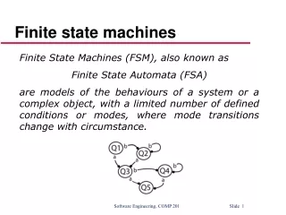
Finite State Models Generative directed models HMMs Naïve Bayes Sequence GeneralGraphs Conditional Conditional Conditional Logistic Regression General CRFs Linear-chain CRFs GeneralGraphs Sequence
Graphical Models Family of probability distributions that factorize in a certain way Directed (Bayes Nets) Undirected (Markov Random Field) Factor Graphs Node is independent of its non-descendants given its parents Node is independent all other nodes given its neighbors
Recap: Naïve Bayes Assumption: features independent given label Generative Classifier Model joint distribution p(x,y) Inference Learning: counting Example П П Labels of neighboring words dependent! The article appeared in the Seattle Times. city? Need to consider sequence! length capitalization suffix
Hidden Markov Models Generative Sequence Model 2 assumptions to make joint distribution tractable 1. Each state depends only on its immediate predecessor.2. Each observation depends only on current state. Finite state model state sequence other person … y1 y2 y3 y4 y5 y6 y7 y8 location other observation sequence x1 x2 x3 x4 x5 x6 x7 x8 person person Yesterday Pedro … Graphical Model yt-1 transitions … … observations
Hidden Markov Models Generative Sequence Model Model Parameters Start state probabilities Transition probabilities Observation probabilities Finite state model state sequence other person … y1 y2 y3 y4 y5 y6 y7 y8 location other observation sequence x1 x2 x3 x4 x5 x6 x7 x8 person person Yesterday Pedro … Graphical Model П transitions - … … observations -
IE with Hidden Markov Models Given a sequence of observations: Yesterday Pedro Domingos spoke this example sentence. and a trained HMM: person name location name background Find the most likely state sequence: (Viterbi) YesterdayPedro Domingosspoke this example sentence. Any words said to be generated by the designated “person name” state extract as a person name: Person name: Pedro Domingos Slide by Cohen & McCallum
IE with Hidden Markov Models For sparse extraction tasks : Separate HMM for each type of target Each HMM should Model entire document Consist of target and non-target states Not necessarily fully connected 18 Slide by Okan Basegmez
Information Extraction with HMMs Example – Research Paper Headers 19 Slide by Okan Basegmez
HMM Example: “Nymble” [Bikel, et al 1998], [BBN “IdentiFinder”] Task: Named Entity Extraction Transitionprobabilities Observationprobabilities Person end-of-sentence - - start-of-sentence - Org or - (Five other name classes) Back-off to: Back-off to: - Other Train on ~500k words of news wire text. Results: Case Language F1 . Mixed English 93% Upper English 91% Mixed Spanish 90% Other examples of shrinkage for HMMs in IE: [Freitag and McCallum ‘99] Slide by Cohen & McCallum
A parse of a sequence 1 1 1 1 … 2 2 2 2 … … … … … K K K K … Given a sequence x = x1……xN, A parse of o is a sequence of states y = y1, ……, yN person 1 2 2 other K location x1 x2 x3 xK Slide by Serafim Batzoglou
Question #1 – Evaluation GIVEN A sequence of observations x1 x2 x3 x4 ……xN A trained HMM θ=( , , ) QUESTION How likely is this sequence, given our HMM ? P(x, θ) - Why do we care? Need it for learning to choose among competing models!
Question #2 - Decoding GIVEN A sequence of observations x1 x2 x3 x4 ……xN A trained HMM θ=( , , ) QUESTION How dow we choose the corresponding parse (state sequence) y1 y2 y3 y4 ……yN, which “best” explains x1 x2 x3 x4 ……xN ? - There are several reasonable optimality criteria: single optimal sequence, average statistics for individual states, …
Question #3 - Learning GIVEN A sequence of observations x1 x2 x3 x4 ……xN QUESTION How do we learn the model parameters θ=( , , ) to maximize P(x, λ) ? -
Solution to #1: Evaluation Given observations x=x1 …xNand HMM θ, what is p(x) ? Naïve: enumerate every possible state sequence y=y1 …yN Probability of x and given particular y Probability of particular y Summing over all possible state sequences we get П 2T multiplications per sequence П For small HMMs T=10, N=10 there are 10 billion sequences! NT state sequences!
Solution to #1: Evaluation Use Dynamic Programming: Define forward variable probability that at time t - the state is yi - the partial observation sequence x=x1 …xthas been emitted
Solution to #1: Evaluation Use Dynamic Programming Cache and reuse inner sums Define forward variables y П - y - - - - - - - - probability that at time t • the state is yt=Si • the partial observation sequence x=x1 …xthas been emitted
The Forward Algorithm INITIALIZATION INDUCTION TERMINATION - - Time: O(K2N) Space: O(KN) K = |S| #states N length of sequence
The Backward Algorithm INITIALIZATION INDUCTION TERMINATION Time: O(K2N) Space: O(KN)
Solution to #2 - Decoding Given x=x1 …xNand HMM θ, what is “best” parse y1 …yN? Several optimal solutions 1. States which are individually most likely: most likely state y*t at time t is then But some transitions may have 0 probability!
Solution to #2 - Decoding Given x=x1 …xNand HMM θ, what is “best” parse y1 …yN? Several optimal solutions 1. States which are individually most likely 2. Single best state sequenceWe want to find sequence y1 …yN, such that P(x,y) is maximized y* = argmaxy P( x, y ) Again, we can use dynamic programming! 1 1 1 1 … 1 2 2 2 2 … 2 2 … … … … K K K K … K o1 o2 o3 oK
The Viterbi Algorithm DEFINE INITIALIZATION INDUCTION TERMINATION buggy Backtracking to get state sequence y*
The Viterbi Algorithm x1 x2 ……xj-1 xj……………………………..xT State 1 Max 2 δj(i) i K Time: O(K2T) Space: O(KT) Linear in length of sequence Remember: δk(i) = probability of most likely state seq ending with state Sk Slides from Serafim Batzoglou
The Viterbi Algorithm Pedro Domingos 36
Solution to #3 - Learning Given x1 …xN, how do we learn θ=( , , ) to maximize P(x)? Unfortunately, there is no known way to analytically find a global maximum θ* such thatθ* = arg max P(o | θ) But it is possible to find a local maximum; given an initial model θ, we can always find a model θ’ such that P(o | θ’) ≥ P(o | θ)
Solution to #3 - Learning Use hill-climbing Called the forward-backward (or Baum/Welch) algorithm Idea Use an initial parameter instantiation Loop Compute the forward and backward probabilities for given model parameters and our observations Re-estimate the parameters Until estimates don’t change much
Expectation Maximization The forward-backward algorithm is an instance of the more general EM algorithm The E Step: Compute the forward and backward probabilities for given model parameters and our observations The M Step: Re-estimate the model parameters
Chicken & Egg Problem If we knew the actual sequence of states It would be easy to learn transition and emission probabilities But we can’t observe states, so we don’t! • If we knew transition & emission probabilities • Then it’d be easy to estimate the sequence of states (Viterbi) • But we don’t know them! 40 Slide by Daniel S. Weld
Simplest Version Mixture of two distributions Know: form of distribution & variance, % =5 Just need mean of each distribution .01 .03 .05 .07 .09 41 Slide by Daniel S. Weld
Input Looks Like .01 .03 .05 .07 .09 42 Slide by Daniel S. Weld
We Want to Predict ? .01 .03 .05 .07 .09 43 Slide by Daniel S. Weld
Chicken & Egg Note that coloring instances would be easy if we knew Gausians…. .01 .03 .05 .07 .09 44 Slide by Daniel S. Weld
Chicken & Egg And finding the Gausians would be easy If we knew the coloring .01 .03 .05 .07 .09 45 Slide by Daniel S. Weld
Expectation Maximization (EM) Pretend we do know the parameters Initialize randomly: set 1=?; 2=? .01 .03 .05 .07 .09 46 Slide by Daniel S. Weld
Expectation Maximization (EM) Pretend we do know the parameters Initialize randomly [E step]Compute probability of instance having each possible value of the hidden variable .01 .03 .05 .07 .09 47 Slide by Daniel S. Weld
Expectation Maximization (EM) Pretend we do know the parameters Initialize randomly [E step]Compute probability of instance having each possible value of the hidden variable .01 .03 .05 .07 .09 48 Slide by Daniel S. Weld
Expectation Maximization (EM) Pretend we do know the parameters Initialize randomly [E step]Compute probability of instance having each possible value of the hidden variable [M step] Treating each instance as fractionally having both values compute the new parameter values .01 .03 .05 .07 .09 49 Slide by Daniel S. Weld
ML Mean of Single Gaussian Uml = argminui(xi – u)2 .01 .03 .05 .07 .09 50 Slide by Daniel S. Weld