Chapter 10
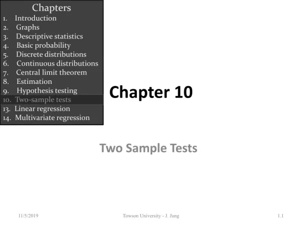
Chapters 1. Introduction 2. Graphs 3. Descriptive statistics 4. Basic probability 5. Discrete distributions 6. Continuous distributions 7. Central limit theorem 8. Estimation 9. Hypothesis testing 10. Two-sample tests 13. Linear regression

Chapter 10
E N D
Presentation Transcript
Chapters 1. Introduction 2. Graphs 3. Descriptive statistics 4. Basic probability 5. Discrete distributions 6. Continuous distributions 7. Central limit theorem 8. Estimation 9. Hypothesis testing 10. Two-sample tests 13. Linear regression 14. Multivariate regression Chapter 10 Two Sample Tests Towson University - J. Jung
Comparing Two Populations Previously we looked at techniques to estimate and test parameters for one population: Population Mean: µ Population Proportion: We will still consider these parameters when we are looking at two populations, however our interest will now be: The difference between two means. The ratio of two variances. The difference between two proportions.
Population 1 Sample: n1 Statistics: Parameters: Difference between Two Means • In order to test and estimate the difference between two population means, we draw random samples from each of two populations. • Initially, we will consider independent samples, that is, samples that are completely unrelated to one another. (Likewise, we consider for Population 2)
Difference between Two Means Because we are comparing two population means, we use the statistic: which is an unbiased and consistent estimator of: µ1- µ2
Sampling Distribution of Differences of Means • is normally distributed if the original populations are normal –or– approximately normal if the populations are non-normal and the sample sizes are large (n1, n2 > 30)!! (Remember condition for CLT) • The expected value of is: • The variance of is: and the standard error is :
Making Inferences About μ1-μ2 • Since is normally distributed if the original populations are normal –or– approximately normal if the populations are non-normal and the sample sizes are large, then: is a N(0,1) (or approximately normal) random variable. • We could use this to build the test statistic and the confidence interval estimator for.
Making Inferences About …except that, in practice, the z statistic is rarely used since the population variances are unknown. • Instead we use a t-statistic. We consider two cases for the unknown population variances: • when we believe they are equal: • when we believe they are not equal: ??
Test Statistic for (equal variances: ) Calculate – the pooled variance estimator as… …and use it here: degrees of freedom
CI Estimator for μ1-μ2 (equal variances) The confidence interval estimator for μ1-μ2 when the population variances are equal is given by: pooled variance estimator degrees of freedom
0 Test Statistic for (unequal variances: ) The test statistic for μ1-μ2 when the population variances are unequal is given by: Likewise, the confidence interval estimator is: degrees of freedom
≥ 0 Which test to use? • Which test statistic do we use? Equal variance or unequal variance? • Whenever there is insufficient evidence that the variances are unequal, it is preferable to perform the equal variances t-test. • This is so, because for any two given samples: The number of degrees of freedom for the equal variances case The number of degrees of freedom for the unequal variances case Larger numbers of degrees of freedom have the same effect as having larger sample sizes ≥
Example • Millions of investors buy mutual funds choosing from thousands of possibilities. • Some funds can be purchased directly from banks or other financial institutions while others must be purchased through brokers, who charge a fee for this service. • This raises the question, can investors do better by buying mutual funds directly than by purchasing mutual funds through brokers.
Example • To help answer this question a group of researchers randomly sampled the annual returns from mutual funds that can be acquired directly and mutual funds that are bought through brokers and recorded the net annual returns, which are the returns on investment after deducting all relevant fees. • Can we conclude at the 5% significance level that directly-purchased mutual funds outperform mutual funds bought through brokers?
Example • To answer the question we need to compare the population of returns from direct and the returns from broker- bought mutual funds. • The data are obviously interval (we've recorded real numbers). • This problem objective - data type combination tells us that the parameter to be tested is the difference between two means µ1- µ2.
Example • The hypothesis to be tested is that the mean net annual return from directly-purchased mutual funds (µ1) is larger than the mean of broker-purchased funds (µ2). • Hence the alternative hypothesis is H1: µ1- µ2 > 0 and H0: µ1- µ2 = 0 • To decide which of the t-tests of µ1 - µ2 to apply we conduct the F-test of σ12/ σ22. (Not covered in class, so just roll with it for now)
Example • Assume F-test concluded that there is not enough evidence to infer that the population variances differ. • It follows that we must apply the equal-variances t-test of µ1- µ2
Example: Result • The value of the test statistic is 2.29. The one-tail p-value is .0122. • We observe that the p-value of the test is small (and the test statistic falls into the rejection region). • As a result we conclude that there is sufficient evidence to infer that on average directly-purchased mutual funds outperform broker-purchased mutual funds
Confidence Interval Estimator • Suppose we wanted to compute a 95% confidence interval estimate of the difference between mean caloric intake for consumers and non-consumers of high-fiber cereals. • The unequal-variances estimator is
Confidence Interval Estimator • We estimate that the return on directly purchased mutual funds is on average between .39 and 5.43 percentage points larger than broker-purchased mutual funds.

