Estimating Rate Constants in Cell Cycle Models for Accurate Simulation of Experimental Data
10 likes | 165 Vues
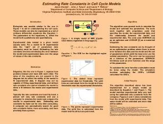
This study explores a computational approach to estimate rate constants in cell cycle models, crucial for simulating biological processes. Using a combination of optimization algorithms and numerical integration (ODRPACK and LSODAR), the research aims to minimize the error between model predictions and experimental data. Initial results demonstrate that the automated estimation effectively identifies parameters that lead to a strong model fit, significantly enhancing the efficiency compared to manual methods. The implications of accurate rate constant estimation for understanding protein interactions in the cell cycle are discussed.

Estimating Rate Constants in Cell Cycle Models for Accurate Simulation of Experimental Data
E N D
Presentation Transcript
Estimating Rate Constants in Cell Cycle Models Jason Zwolak1, John J. Tyson2, and Layne T. Watson1 1Department of Computer Science and 2Department of Biology Virginia Polytechnic Institute and State University, Blacksburg, VA 24061-0106 jzwolak@vt.edu, Tel: 540-231-5958 Cdc25 Cdc2 Cdc2 Cdc2 Cdc2 Cdc2 P Cyclin Cyclin Cyclin Cyclin Wee1 Cyclin Introduction Biologists use models similar to the one in Figure 1 to aid in understanding the cell cycle. These models can also be expressed as a set of ordinary differential equations like Equation 1. The parameters to the equations, k*, affect the model both qualitatively and quantitatively. Experimental data related to a given model usually exist. For a model to fit experimental data the "right" set of parameters (rate constants) must be found. Estimating the rate constants involves minimizing the error between the model and experimental data over the range of values of the rate constants. Algorithm The algorithm uses general tools to simulate the model and estimate the parameters. The tools work together with proprietary code that specifies the model, the experimental data, and the relationship between the model and experimental data. The code uses ODRPACK [2] as an optimizer and LSODAR [3] as a numerical integrator. Estimating the rate constants can be thought of as an optimization problem where there is some error between the data and the model and the set of parameters which yield the least error are the optimal parameters. The error can be expressed as a function of the parameters. ODRPACK minimizes such an error function over the range of the parameters. To calculate the error function a simulation must be done using the model. The simulation involves calculating the ODE's. LSODAR calculates the ODE's. Figure 1. A simple model of MPF (Cyclin-Cdc2 dimer) regulation in frog eggs [1]. Equation 1. The ODE for the highlighted region of Figure 1. Motivation Diagrams, like the one in Figure 1, express how proteins interact and react with each other. The rates of the reactions are not present in the diagram but do affect the ability of the model to fit experimental data. A diagram may not be capable of fitting experimental data, and without rate constants one cannot simulate the model to show a fit between the model and experimental data. Typically the rate constants are found by hand: a person will vary rate constants and use a computer to simulate the model and compare the results to experimental data. Estimating rate constants by hand can be very time consuming. A computer can automatically search for good rate constants faster, more accurately, and more precisely than a person. . Figure 2. The dotted lines represent experimental data for thresholds. The solid lines are calculated from the model and have thresholds near the experimental thresholds. Initial Results The algorithm described above has been implemented for a simple model as described by Equation 1 and Figure 1. The model matches experimental data very well using the estimated rate constants from the computer. Figures 2 and 3 show calculations from the model with experimental data. This same model will be extended and more data will be added. References: 1. Tyson, J.J.; B. Novak; K. Chen; J. Val. 1995. Checkpoints in the cell cycle from a modeler's perspective. Progress in Cell Cycle Research 1, 1-8. 2. Boggs, P.T.; R.H. Byrd; J.E. Rogers; R.B. Schnabel. 1992. User's Reference Guide for ODRPACK Version 2.01: Software for Weighted Orthogonal Distance Regression. Center for Computing and Applied Mathematics, U.S. Department of Commerce, Gaithersburg, MD. 3. Hindmarsh, A.C. 1983. ODEPACK: A Systematized Collection of ODE Solvers. Scientific Computing (R.S. Stepleman, et al., eds.). North Holland Publishing Co., New York, 55--64. Figure 3. The points represent experimental data. The solid line is calculated from the model and fits all but one point well.