The Course
The Course. Books Computer Vision – Adrian Lowe Digital Image Processing – Gonzalez, Woods Image Processing, Analysis and Machine Vision – Milan Sonka, Roger Boyle. Image representation Image statistics Histograms ( frequency ) Entropy ( information )

The Course
E N D
Presentation Transcript
The Course • Books • Computer Vision – Adrian Lowe • Digital Image Processing – Gonzalez, Woods • Image Processing, Analysis and Machine Vision – Milan Sonka, Roger Boyle • Image representation • Image statistics • Histograms (frequency) • Entropy (information) • Filters (low, high, edge, smooth)
Digital Image Processing • Human vision - perceive and understand world • Computer vision, Image Understanding / Interpretation, Image processing. • 3D world -> sensors (TV cameras) -> 2D images • Dimension reduction -> loss of information • low level image processing • transform of one image to another • high level image understanding • knowledge based - imitate human cognition • make decisions according to information in image
Acquisition, preprocessing no intelligence Extraction, edge joining Recognition, interpretation intelligent Introduction to Digital Image Processing
Low level digital image processing • Low level computer vision ~ digital image processing • Image Acquisition • image captured by a sensor (TV camera) and digitized • Preprocessing • suppresses noise (image pre-processing) • enhances some object features - relevant to understanding the image • edge extraction, smoothing, thresholding etc. • Image segmentation • separate objects from the image background • colour segmentation, region growing, edge linking etc • Object description and classification • after segmentation
Signals and Functions • What is an image • Signal = function (variable with physical meaning) • one-dimensional (e.g. dependent on time) • two-dimensional (e.g. images dependent on two co-ordinates in a plane) • three-dimensional (e.g. describing an object in space) • higher-dimensional • Scalar functions • sufficient to describe a monochromatic image - intensity images • Vector functions • represent color images - three component colors
Image Functions • Image - continuous function of a number of variables • Co-ordinates x, y in a spatial plane • for image sequences - variable (time) t • Image function value = brightness at image points • other physical quantities • temperature, pressure distribution, distance from the observer • Image on the human eye retina / TV camera sensor - intrinsically 2D • 2D image using brightness points = intensity image • Mapping 3D real world -> 2D image • 2D intensity image = perspective projection of the 3D scene • information lost - transformation is not one-to-one • geometric problem - information recovery • understanding brightness info
Image Acquisition & Manipulation • Analogue camera • frame grabber • video capture card • Digital camera / video recorder • Capture rate 30 frames / second • HVS persistence of vision • Computer, digitised image, software (usually c) • f(x,y) #define M 128 #define N 128 unsigned char f[N][M] • 2D array of size N*M • Each element contains an intensity value
Image definition • Image definition: • A 2D function obtained by sensing a scene • F(x,y), F(x1,x2), F(x) • F - intensity, grey level • x,y - spatial co-ordinates • No. of grey levels, L = 2B • B = no. of bits
Brightness and 2D images • Brightness dependent several factors • object surface reflectance properties • surface material, microstructure and marking • illumination properties • object surface orientation with respect to a viewer and light source • Some Scientific / technical disciplines work with 2D images directly • image of flat specimen viewed by a microscope with transparent illumination • character drawn on a sheet of paper • image of a fingerprint
Monochromatic images • Image processing - static images - time t is constant • Monochromatic static image - continuous image function f(x,y) • arguments - two co-ordinates (x,y) • Digital image functions - represented by matrices • co-ordinates = integer numbers • Cartesian (horizontal x axis, vertical y axis) • OR (row, column) matrices • Monochromatic image function range • lowest value - black • highest value - white • Limited brightness values = gray levels
Chromatic images • Colour • Represented by vector not scalar • Red, Green, Blue (RGB) • Hue, Saturation, Value (HSV) • luminance, chrominance (Yuv , Luv) S=0 Green Hue degrees: Red, 0 deg Green 120 deg Blue 240 deg Red Green V=0
Image quality • Quality of digital image proportional to: • spatial resolution • proximity of image samples in image plane • spectral resolution • bandwidth of light frequencies captured by sensor • radiometric resolution • number of distinguishable gray levels • time resolution • interval between time samples at which images captured
Image summary • F(xi,yj) • i = 0 --> N-1 • j = 0 --> M-1 • N*M = spatial resolution, size of image • L = intensity levels, grey levels • B = no. of bits
Digital Image Storage • Stored in two parts • header • width, height … cookie. • Cookie is an indicator of what type of image file • data • uncompressed, compressed, ascii, binary. • File types • JPEG, BMP, PPM.
PPM, Portable Pixel Map • Cookie • Px • Where x is: • 1 - (ascii) binary image (black & white, 0 & 1) • 2 - (ascii) grey-scale image (monochromic) • 3 - (ascii) colour (RGB) • 4 - (binary) binary image • 5 - (binary) grey-scale image (monochromatic) • 6 - (binary) colour (RGB)
PPM example • PPM colour file RGB P3 # feep.ppm 4 4 15 0 0 0 0 0 0 0 0 0 15 0 15 0 0 0 0 15 7 0 0 0 0 0 0 0 0 0 0 0 0 0 15 7 0 0 0 15 0 15 0 0 0 0 0 0 0 0 0
Image statistics • MEAN = • VARIANCE2 = • STANDARDEVIATION =
Histograms, h(l) • Counts the number of occurrences of each grey level in an image • l = 0,1,2,… L-1 • l = grey level, intensity level • L = maximum grey level, typically 256 • Area under histogram • Total number of pixels N*M • unimodal, bimodal, multi-modal, dark, light, low contrast, high contrast
Probability Density Functions, p(l) • Limits 0 < p(l) < 1 • p(l) = h(l) / n • n = N*M (total number of pixels)
Histogram Equalisation, E(l) • Increases dynamic range of an image • Enhances contrast of image to cover all possible grey levels • Ideal histogram = flat • same no. of pixels at each grey level • Ideal no. of pixels at each grey level =
Histogram equalisation Typical histogram Ideal histogram
E(l) Algorithm • Allocate pixel with lowest grey level in old image to 0 in new image • If new grey level 0 has less than ideal no. of pixels, allocate pixels at next lowest grey level in old image also to grey level 0 in new image • When grey level 0 in new image has > ideal no. of pixels move up to next grey level and use same algorithm • Start with any unallocated pixels that have the lowest grey level in the old image • If earlier allocation of pixels already gives grey level 0 in new imageTWICE its fair share of pixels, it means it has also used up its quota for grey level 1 in new image • Therefore, ignore new grey level one and start at grey level 2 …..
Simplified Formula • E(l) equalised function • max maximum dynamic range • round round to the nearest integer (up or down) • L no. of grey levels • N*M size of image • t(l) accumulated frequencies
Histogram equalisation examples Typical histogram After histogram equalisation
Before HE After HE Ideal=3 Histogram Equalisation e.g.
Noise in images • Images often degraded by random noise • image capture, transmission, processing • dependent or independent of image content • White noise - constant power spectrum • intensity does not decrease with increasing frequency • very crude approximation of image noise • Gaussian noise • good approximation of practical noise • Gaussian curve = probability density of random variable • 1D Gaussian noise - µ is the mean • is the standard deviation
Gaussian noise e.g. 50% Gaussian noise
Types of noise • Image transmission • noise usually independent image signal • additive, noise v and image signal g are independent • multiplicative, noise is a function of signal magnitude • impulse noise (saturated = salt and pepper noise)
Data Information • Different quantities of data used to represent same information • people who babble, succinct • Redundancy • if a representation contains data that is not necessary • Compression ratio CR = • Relative data redundancy RD =
Types of redundancy • Coding • if grey levels of image are coded in such away that uses more symbols than is necessary • Inter-pixel • can guess the value of any pixel from its neighbours • Psyco-visual • some information is less important than other info in normal visual processing • Data compression • when one / all forms of redundancy are reduced / removed • data is the means by which information is conveyed
Coding redundancy • Can use histograms to construct codes • Variable length coding reduces bits and gets rid of redundancy • Less bits to represent level with high probability • More bits to represent level with low probability • Takes advantage of probability of events • Images made of regular shaped objects / predictable shape • Objects larger than pixel elements • Therefore certain grey levels are more probable than others • i.e. histograms are NON-UNIFORM • Natural binary coding assigns same bits to all grey levels • Coding redundancy not minimised
Run length coding (RLC) • Represents strings of symbols in an image matrix • FAX machines • records only areas that belong to the object in the image • area represented as a list of lists • Image row described by a sublist • first element = row number • subsequent terms are co-ordinate pairs • first element of a pair is the beginning of a run • second is the end • can have several sequences in each row • Also used in multiple brightness images • in sublist, sequence brightness also recorded
Inter-pixel redundancy, IPR • Correlation between pixels is not used in coding • Correlation due to geometry and structure • Value of any pixel can be predicted from the value of the neighbours • Information carried by one pixel is small • Take 2D visual information • transformed NONVISUAL format • This is called a MAPPING • A REVERSIBLE MAPPING allows original to be reconstructed after MAPPING • Use run-length coding
Psyco-visual redundancy, PVR • Due to properties of human eye • Eye does not respond with equal sensitivity to all visual information (e.g. RGB) • Certain information has less relative importance • If eliminated, quality of image is relatively unaffected • This is because HVS only sensitive to 64 levels • Use fidelity criteria to assess loss of information
In a noiseless channel, the encoder is used to remove any redundancy 2 types of encoding LOSSLESS LOSSY Design concerns Compression ratio, CR achieved Quality achieved Trade off between CR and quality PVR removed, image quality is reduced 2 classes of criteria OBJECTIVE fidelity criteria SUBJECTIVE fidelity criteria OBJECTIVE: if loss is expressed as a function of IP / OP Fidelity Criteria
Input f(x,y) compressed output f(x,y) error e(x,y) = f(x,y) -f(x,y) erms = root mean squared error SNR = signal to noise ratio PSNR = peak signal to noise ratio Fidelity Criteria
How few data are needed to represent an image without loss of info? Measuring information random event, E probability, p(E) units of information, I(E) I(E) = self information of E amount of info is inversely proportional to the probability base of log is the unit of info log2 = binary or bits e.g. p(E) = ½ => 1 bit of information (black and white) Information Theory
Connects source and user physical medium Source generates random symbols from a closed set Each source symbol has a probability of occurrence Source output is a discrete random variable Set of source symbols is the source alphabet Infromation channel
Entropy is the uncertainty of the source Probability of source emitting a symbol, S = p(S) Self information I(S) = -log p(S) For many Si , i = 0, 1, 2, … L-1 Defines the average amount of info obtained by observing a single source output OR average information per source output (bits) alphabet = 26 letters 4.7 bits/letter typical grey scale = 256 levels 8 bits/pixel Entropy
Need templates and convolution Elementary image filters are used enhance certain features de-enhance others edge detect smooth out noise discover shapes in images Convolution of Images essential for image processing template is an array of values placed step by step over image each element placement of template is associated with a pixel in the image can be centre OR top left of template Filters
Each element is multiplied with its corresponding grey level pixel in the image The sum of the results across the whole template is regarded as a pixel grey level in the new image CONVOLUTION --> shift add and multiply Computationally expensive big templates, big images, big time! M*M image, N*N template = M2N2 Template Convolution
Let T(x,y) = (n*m) template Let I(X,,Y) = (N*M) image Convolving T and I gives: CROSS-CORRELATION not CONVOLUTION Real convolution is: convolution often used to mean cross-correlation Convolution
Template is not allowed to shift off end of image Result is therefore smaller than image 2 possibilities pixel placed in top left position of new image pixel placed in centre of template (if there is one) top left is easier to program Periodic Convolution wrap image around a ball template shifts off left, use right pixels Aperiodic Convolution pad result with zeros Result same size as original easier to program Templates
Need templates and convolution Elementary image filters are used enhance certain features de-enhance others edge detect smooth out noise discover shapes in images Convolution of Images essential for image processing template is an array of values placed step by step over image each element placement of template is associated with a pixel in the image can be centre OR top left of template Filters
Each element is multiplied with its corresponding grey level pixel in the image The sum of the results across the whole template is regarded as a pixel grey level in the new image CONVOLUTION --> shift add and multiply Computationally expensive big templates, big images, big time! M*M image, N*N template = M2N2 Template Convolution
Template is not allowed to shift off end of image Result is therefore smaller than image 2 possibilities pixel placed in top left position of new image pixel placed in centre of template (if there is one) top left is easier to program Periodic Convolution wrap image around a ball template shifts off left, use right pixels Aperiodic Convolution pad result with zeros Result same size as original easier to program Templates
Moving average of time series smoothes Average (up/down, left/right) smoothes out sudden changes in pixel values removes noise introduces blurring Classical 3x3 template Removes high frequency components Better filter, weights centre pixel more Low pass filters