Download
1 / 33
330 likes | 486 Vues
Turbulence Modelling of Buoyancy-Affected Flows. Brian Launder UMIST, Manchester, UK. Aims of Lecture. To give an impression of what level of RANS modelling is needed to predict different types of gravity-affected shear flow phenomena

E N D
Turbulence Modelling of Buoyancy-Affected Flows Brian Launder UMIST, Manchester, UK Singapore Turbulence Colloquium
Aims of Lecture • To give an impression of what level of RANS modelling is needed to predict different types of gravity-affected shear flow phenomena • To show some illustrative predictions of buoyant and stratified flow ______________________________ • Even if buoyant/stratified flows are of no interest, much of the lecture has parallels with other agencies modifying turbulence, e.g. system rotation Singapore Turbulence Colloquium
An important distinction • A buoyant flow is one where the main effects of the gravitational vector are on the mean motion. • A stratifiedflow is one where the main effects of the g vector are on the fluctuating motion and thus, after Rey-nolds averaging, on the 2nd moments • Vertical flows are usually “buoyant”; ….horizontal flows usually “stratified”. Singapore Turbulence Colloquium
A modelling consequence • Buoyant flows can often be computed with simple eddy viscosity models… at least close to a wall. • Stratified flows always require at least some form of 2nd-moment closure (perhaps truncated) • …maybe even 3rd-moment or U-RANS modelling to capture the flow behaviour sufficiently closely in extreme stratification Singapore Turbulence Colloquium
Refinements to k-εEVM for (mainly) vertical, buoyant flows near walls • In many simple flows NO refinement needed because shear generation of k (and ε) much larger than buoyant generation. • Note buoyant k-generation is: <ρ’ui>gi/ρ or G = - β<uiθ>gi; β Vol. exp’n coeff • If x2 is vertically up: gi = [0, -g, 0]; Θ = Θ(x1); U=U(x1) • G = + βg<u2θ> = 0 with SGD but … = - cθcμβg(k3/ε2)Θ/x1U2/x1 with GGDH ie. horizontal temp. gradients cause buoyant effects. • This refinement brings (usually minor) improve-ments to vertical flows (e.g. Ince & Launder, 1989) Singapore Turbulence Colloquium
A problem with flow near walls • If source of buoyancy arises through heat transfer through a wall, the wall sub-layer region is principally affected. • Flow is then far from local equilibrium • But equally, for an industrial flow simulation, one needs to avoid using a fine-grid “low-Reynolds-number” model. • Two new wall-function approaches have been developed to remove these problems: PhD’s and papers by Gerasimov and Gant Singapore Turbulence Colloquium
Gerasimov’s analytical wall functions – a recap • Based on a simplified analytical solution of wall-parallel momentum equation assuming a linear eddy viscosity variation over wall cell. • Gravitational term appears in momentum equation and thus affects the form of the wall function. • Vital to include the effects of thickening and thinning of the viscous sublayer. • Reduces computing budget by at least by factor 10 compared the ‘low-Reynolds-number’ treatments. Singapore Turbulence Colloquium
Application to up-flow in a heated pipe with k-ε EVM; Gerasimov(2003) Singapore Turbulence Colloquium
Downward flow in an annulus with core tube heated; Gerasimov (2003) Singapore Turbulence Colloquium
How to extend linear EVM’s to stratified flows? • When a linear EVM is applied to horizontal or recirc-ulating flows, the model is often made sensitive to gravitational influencesthrough the ε-equation. • Typically: Gravitational Source = Cε3Gε/k • Different values taken for Cε3according to whether the flow is horizontal or vertical; stable or unstable… • Others have made Cε3 ~ tanh (vvert/vhoriz) [Fluent] • These approaches are NOT recommended unless extensive calibration against experiments similar to those to be predicted has been made ! Singapore Turbulence Colloquium
Some guidelines in computing stratified flows • Don’t use a linear EVM. • Incorporate primary gravitational effects through constitutive equations for stresses and heat flux • Give the shear and gravitational terms equal weight in the ε equation … unless you are considering just a single flow type and are confident to tune Singapore Turbulence Colloquium
Where does buoyancy enter the turbulence equations? • In the second-moment equations (by way of the Navier Stokes equations): <φDui /Dt> = ….<φρ’ >gi /ρ (where ui is turbulent velocity and denotes uj , θ, etc) … and in the pressure-strain term (see later) • In the length scale or ε equation?? • Our recommended practice is to handle G identically to P in thescale equation… though this matter is not entirely settled. Singapore Turbulence Colloquium
Second moment equations with buoyant terms Singapore Turbulence Colloquium
Why a simple ε-equation fix doesn’t work • Consider a simple shear flow with x1 the flow direction and x2 that of velocity/temp gradient. • If x1 is horizontal, x2 vertical the g vector acts as in upper diagram • If x1is vertical, x2 horiz-ontal, the lower figure shows the g impacts. Singapore Turbulence Colloquium
Features of the transport equations • ‘Invisible’ gravitational effects also act on the pressure fluctuations • Possible effects also in the ε equation • Note <θ2> contains no pressure fluctuations …but εθθhard to model. Usually we assume thermal time scale <θ2>/εθθ is linked to the dynamic time scale… though somewhat affected by anisotropy of the heat flux Singapore Turbulence Colloquium
Buoyant effects on pressure correlations: 1 –Basic Model • The IP model for shear assumes: ij2 = -c2[Pij- ⅔ijP] with c2 0.6 (exact for isotropic turb.) • By analogy we take: ij3 = -c3 [Gij - ⅔ijG] • Now c3 = 0.3 in isotropic turbulence but experiments suggest optimum value in the range 0.5 0.6. • Pressure fluctuations in heat flux equations: i = - c3Gi • Isotropic turbulence suggests c3=⅓ but it is usually taken equal to c3. • Wall-reflection effects must be added but calibration has been done only for an infinite plane wall. Singapore Turbulence Colloquium
Buoyant effects on pressure correlations: 2 – TCL Model • Application of two-component-limit principles to buoyant parts of pressure fluctuations produces forms with NO empirical constants. • The TCL form of ij3 is very long (see Craft & Launder, 2002 in “Closure Strategies” book, p. 411) • i3 = ⅓βgi<2>- βgkaik • Note both ij3 and i3 satisfy isotropic and 2-component limits. • NO wall corrections beyond viscosity affected sublayer Singapore Turbulence Colloquium
Handling the dissipation rates • Standard equation for but with c3 = c1 • For TCL version c1 = 1.0; c2 =1.92/(1.+0.7AA2½) • ….where A2 aijaji and A 1 - (9/8)[A2 – A3] (Lumley’s flatness factor) • Local isotropy and “proportional timescales” for scalars and their fluxes: Singapore Turbulence Colloquium
Modelling the transport terms • Diffusive transport usually handled by GGDH: <uk> = - c<ujuk>(k/)<>/xj • …or it may be simplified to give an algebraic set of equations, e.g Rodi (1971): conv.- diff’n of <> = [conv. - diff’n of k]×{<>/k} = [P - ] <>/k • But situations also arise where transport is very important and then 3rd-moment closure may be necessary. Singapore Turbulence Colloquium
Comparison of spreading rates for plumes Singapore Turbulence Colloquium
Application 1: Downwards directed warm jet into cool “pool” • In practice “pool” moves slowly vertically up to give a steady flow. • Profiles of mean velocity (c) and shear stress (b) better represented by TCL scheme (solid line) than basic model (broken line). • From Cresswell et al (1989) Singapore Turbulence Colloquium
Applications 2: The downwards directed buoyant wall jet • Downward directed warm wall jet collides with slow-moving up-flow which causes jet to turn around. • Buoyant effects important. • LES data of Laurence et al(2003) extend exp’ts by Prof. Jackson’s team. Singapore Turbulence Colloquium
Penetration depth with k- and TCL models versus LES for isothermal flow Singapore Turbulence Colloquium
Turbulence energy using 2nd moment closure – buoyant case • Basic 2nd moment closure no better than k-ε EVM • TCL model mimics turbulence energy levels much better Singapore Turbulence Colloquium
Buoyant flow: predicted temperature field with k- model • Too little mixing predicted by all forms so high temperatures (red) remain longer. • Again “standard” WF’s far different from “low-Re” result even though no heat transfer through the wall Singapore Turbulence Colloquium
2nd moment closure predictions of thermal field • “Basic model shows too little mixing and too deep penetration with St. WF • TCL-AWF gives most rapid mixing, closest to experiment Singapore Turbulence Colloquium
Comparison with LES thermal field Singapore Turbulence Colloquium
Application 3:Stably stratified mixing layerNB:k- EVM creates far too much mixing but the two 2nd moment closures exhibit unphysical over- and under-shoots due to inadequate diffusion model Singapore Turbulence Colloquium
Stratified mixing layer -2 • Kidger (1999) developed 3rd moment closure for components containing the density fluctuations, e.g. • P1, P2, G: generation by 1st, 2ndmoments and gravitational effects. pressure interactions, etc. • For further details of modelling see Launder & Sandham (2002) pp 417 - 418 Singapore Turbulence Colloquium
Stratified mixing layer - 3:TCL 2nd and 3rd moment closures compared Singapore Turbulence Colloquium
Conclusions -1 • Different levels of modelling are needed for buoyant and stratified flows. • Low-Re k- modelling successful for buoyant up- and down-flow in pipes and channels (but make sure Ret k2/ not yk½/) • Gerasimov’s analytical wall functions perform well in such flows, saving typically 90% of the computer time • Buoyantly modified vertical free shear flows (plumes) not well modelled at this level Singapore Turbulence Colloquium
Conclusions 2 • The TCL model mimics observed behaviour in free buoyant flows and stratified flow … consistent with earlier non-buoyant predictions. • Force field effects on diffusion of second moments may be critically important. Then it may be essential to adopt (at least a partial) third-moment modelling. • Other strategies include U-RANS treatment for unstable buoyant flows (see Prof Hanjalić’s lectures). Singapore Turbulence Colloquium