Spatial Data Mining

1. Spatial Data Mining • Data mining is a process of knowledge discovery related to finding patterns of interest within a large data set. • Examples of databases where spatial data mining is useful are: • Earth Observation Satellites (terabyte per day) • Census • Weather systems • Marketing • so on….

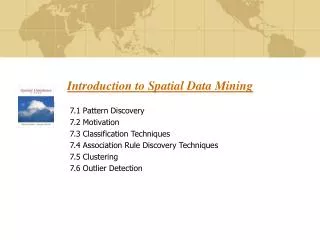
2. Examples of Spatial Patterns • Historic Examples • 1855 Asiatic Cholera in London : A water pump identified as the source… Modern Examples • Cancer clusters to investigate environment health hazards… • Crime hotspots for planning police patrol routes… • Bald eagles nest on tall trees near open water… • Unusual warming of Pacific ocean (El Nino)

3. Spatial Data Mining • Data mining is a combination of processes : • Data extraction • Data clean • Selection of characteristics • Algorithms • Analysis of results • Important characteristic to explore for spatial data mining: similar objects tend to be spatially close.

4. Data Mining: Process DB Association Clustering Classification Expert Analyst Problem adjustment technique action interpretation feedback Algorithms Data Mining OGIS SQL Verification Refinement Visualization Hypothesis DB

5. Statistics versus Data Mining • Data mining is strongly related to statistical analysis. • Data mining can be seen as a filter (exploratory data analysis) before applying a rigorous statistical tool. • Data mining generates hypothesis that are then verified. • The filtering process do not guarantee completeness (wrong elimination or missing).

6. A Classification of Data Mining Processes • The three most common process of data mining are: • Association rules: Determination of interaction between attributes. For example: • X Y: • Classification: Estimation of the attribute of an entity in terms of attribute values of another entity. Some applications are: • Predicting locations (shopping centers, habitat, crime zones) • Thematic classification (satellite images) • Clustering: It is a form of learning without supervision, where classes and the number of classes are unknown. Applications:

7. Association Rules • A spatial association rule is a rule indicating certain association relationship among a set of spatial and possibly some non-spatial predicates. Example: “Most big cities in Canada are close to the Canada­U.S. border” A strong rule indicates that the patterns in the rule have relatively frequent occurrences in the database and strong implication relationships.

8. Association Rules • Spatial association rules are defined in terms of spatial predicates: P1 P2 …  P1   Q1 Q2…  Qm For example: is_a(x, country)  close(x,Mediterranean) s%,c% is(x, wine - exporter) where for i1  i2: s%: i1and i2occur at least s% of cases c%: among all cases when i1 occurs, at least c% of the times i2 also occurs.

9. Association Rules: A priori • Principle: If an item set has a high support, then so do all its subsets. • The steps of the algorithm is as follows: • first,discover all 1-itemsets that are frequent • combine to form 2-itemsets and analyze for frequent set • go on until no more itemsets exceed the therehold. • search for rules

10. Association Rules: A priori Cases items D A V C A T C D A V C D A T C D A T V C A T V CD D Alarm A TV T VCR V Computador C

11. Association Rules : A priori Frequency of itemsets 100% (6) A 83% (5) C, A C 67 % (5) C, T, V, D A DC,AT,AV,DAC 50% (3) DV,TC,VC,DAV, DVC,ATC,AVC, DAVC

12. Association Rules: A priori Confidence of association rules = 100% D  A (4/4) D  C (4/4) D  AC (4/4) T  C (4/4) V  A (4/4) C  A (5/5) D  A (4/4) D  A (3/3) D  A (3/3) D  A (4/4) D  A (3/3) D  A (3/3) VC  A (3/3) DV  A (3/3) VC  A (3/3) DAV  A (3/3) DVC  A (3/3) AVC  A (3/3) Association rules with confidence >= 80% C  D (4/5) A  C (5/6) C DA(4/5)

13. Association rules • Differences with respect to spatial domain: • The notion of transaction or case does not exist, since data are immerse in a continuous space.The partition of the space may introduce errors with respect to overestimation or subestimation confidences. • The size of itemsets is less in the spatial domain. Thus, the cost of generating candidate is not a dominant factor. The enumeration of neighbors dominates the final computational cost. • In most cases, the spatial items are discrete version of continuous variables. • The notion of transaction is replaced by neighborhood.

14. Discovery of Spatial Association Rules (cont.) Example GeoMiner query: discover spatial association rules inside British Columbia from road R, water W, mines M, boundary B in relevance to town T where g_close_to(T.geo, X.geo) and X in {R, W, M, B} and T.type = “large” and R.type in {divided_highway} and W.type in {sea, ocean, large_lake, large_river} and B.admin_region_1 in “B.C.”and B.admin_region_2 in “U.S.A.”

15. X is close_to Y, if their distance is within 80 kms X is a town and Y is a country then Discovery of Spatial Association Rules (cont.) Note: “close_to” is a condition­dependent predicate and is defined by a set of knowledge rules. For example, the following rule states: Rule: close_to(X,Y )  is_a(X, town)  is_a(Y, country)  dist(X, Y, d)  d = 80 km

16. g_close_to Water Not_disjoint Close_to Sea River Lake Intersects Inside Equal Contains Large river Small river Adjacent to Covered by Covers Fraser river Intersects Inside Contains Discovery of Spatial Association Rules (cont.) Level 1 2 3 4 Hierarchy for data relations Hierarchy of topological relations

17. The set of relevant data is retrieved by execution of the data retrieval methods of the data mining query, which extracts the following data sets whose spatial portion is inside B.C.: Discovery of Spatial Association Rules (cont.) Step 1: Task_relevant_DB := extract task relevant objects(SDB, RDB); ... g_close_to(T.geo, X.geo) and X in {R, W, M, B} and T.type = “large” and R.type in {divided_highway}and W.type in {sea, ocean, large_lake, large_river} and B.admin_region_1 in “B.C.”and B.admin_region_2 in “U.S.A.” ... Towns Roads Water Mines boundary only large towns; only divided highways 2 ; only seas, oceans, large lakes and large rivers; any mines; only the boundary of B.C., and U.S.A.

18. The “generalized_close_to” (g_close_to) relationship between (large) towns and the other four classes of entities is computed at a relatively coarse resolution level. [MBR data structure or R*­trees and other approximations] – Later… Discovery of Spatial Association Rules (cont.) Step 2: Coarse_predicate_DB := coarse spatial computation(Task_relevant_DB); At this level we can already mine: is_a(X, large_town)  g_close_to(X, water): (80%) is_a(X, large_town)  g_close_to(X, sea)  g_close_to (X, us_boundary):(92%)

19. Refined computation is performed on the large predicate sets, i.e., those retained in the g_close_to table. Each g_close_to predicate is replaced by one or a set of concrete predicate(s) such as intersect, adjacent_to, close_to, inside, etc. Discovery of Spatial Association Rules (cont.) Step 3: Large_Coarse_predicate_DB := filtering_with_min_support(Coarse predicate DB);

20. The level­by­level detailed computation of large predicates and the corresponding association rules is presented as follows. The computation starts at the top­most concept level and computes large predicates at this level. Discovery of Spatial Association Rules (cont.) Step 4: Large_Coarse_predicate_DB := filtering_with_min_support(Coarse predicate DB); Min support = 20 for level 1

21. After mining rules at the highest level of the concept hierarchy, large k­predicates can be computed in the same way at the lower concept levels, which results in tables Discovery of Spatial Association Rules (cont.) Step 5: Find large predicates and mine rules(Fine_predicate_DB); Level 2: Min support = 10 for level 2

22. Discovery of Spatial Association Rules (cont.) Min support = 7 for level 3 Level 3: A rule example: is_a(X, large town)  adjacent(X, sea)  close_to (X, us_boundary) : (100%) The mining process stops at the lowest level of the hierarchies or when an empty large 1­predicate set is derived.

23. Classification and Regression • Classification: • constructs a model (classifier) based on the training set and uses it in classifying new data • Example: Climate Classification,… • Regression: • models continuous-valued functions, i.e., predicts unknown or missing values • Example: stock trends prediction,…

24. Classification • Definition  : D  L where D is the domain of , i.e., the domain of attribute values and L is the set of levels or classes. For example, in a problem of habitat of birds, D is a space of three dimensions: longevity of the vegetation, depth of water, and distance to water. L has two possible values: nest and no nest. • The goal is to find a good .

25. Training Data Training Data Classifier (Model) Classification (1): Model Construction Classification Algorithms IF rank = ‘professor’ OR years > 6 THEN tenured = ‘yes’

26. Classifier Testing Data Unseen Data Classification (2): Prediction Using the Model (Jeff, Professor, 4) Tenured?

27. Classification Techniques • Decision Tree Induction • Bayesian Classification • Neural Networks • Genetic Algorithms • Fuzzy Set and Logic

28. Regression • Regression is similar to classification • First, construct a model • Second, use model to predict unknown value • Methods • Linear and multiple regression • Non-linear regression • Regression is different from classification • Classification refers to predict categorical class label • Regression models continuous-valued functions

29. Predicting Location Using Similarity Map • Given: • S is a set of locations { s1,…sn} in a geographic space G. • A collection of exploratory functions xk : S  Rk, where Rk , k = 1 .. K, is the range of possible values for the exploratory functions. • A dependent class variable c : S  C= c1,..cM • A value for parameter , the relative importance of spatial accuracy. • Find: classification model: c : R1 x …Rk C • Objective: Maximize similarity (map si  S (c (x1,… xk)),map(c )) = (1- ) classification accuracy(c , c) +  spatial accuracy (c , c)

30. Predicting Locations Using Similarity Map • Constraints: • the geographic space S is the Euclidean space • The values of exploratory functions, x1.. xk , dependent classvariable, c , can depend on the neighbors’ values (spatial auto-correlation) • The domain Rk of the exploratory ina domain of real numbers • The domain of dependent variable C = {0,1}. • Two characteristics: • Spatial autocorrelation • The objective function combines spatial and classification accuracy.

31. Clustering • It is the process of finding groups, without knowing in advance the number and the labels of the groups. • Examples: the counties in Chile can be clustered based on 4 attributes: • Porcentaje de desempleo • Población • Ingreso por cápita • Expectativa de vida • Two types of clustering with different objectives are: • Identify the central cities and their influence region by means of the variance of the attribute values within the space. • Identify areas in the space where an attribute is homogeneous,

32. Clustering • Definition 1: • Given a set of S = {s1,..sn} spatial objects (ex., points) and a real valued no spatial attribute evaluated over S (: S  R). • Find two disjoint subsets S, C and NC = S - C, whereC = {s1,…,sk}, NC = {nc1,…,ncl} y k < n • Goal min C S ∑l j=1 | (ncj) - ∑k i=1 ((ci )/dist(ncj,ci))|2 • where dist(a,b) is the Euclidian distance or some distance measure Constraints: • It satisfies that the influence of the center decreases with the square of the distance • There is at most one non spatial attribute

33. Clustering • Definition 2: • Given a set of S = {s1,..sn} spatial objects objests, a set of real valued no spatial attributes i,con i = 1,… I defined over S (k: S  R) and a structure of neighborhood E in S. • Find K subsets Ck S, with k = 1 .. K, such that • Goal min CkS ∑ck,si Ck,sj Ck dist(F(si),F(sj))+ ∑I,j nbddist(Ci,Cj) • whereF is the cross product of ’is, I = 1..n; dist(a,b) is the distance measure and nbddist(C,D) is the number of points in C andD that belong to E, I.e., pair of neighbors mapped to different clusters. • Constraints: |Ck| > 1 for all k = 1 .. K

34. Clustering: categories • Hierarchical methods:Starting with a cluster, successive partitions are made until a criterion is satisfied. These algorithms result in a tree of clusters called dendograms. • Partitional: It considers each pattern as a cluster and then, reallocate data in each cluster until a criterion is satisfied. This methods tend to find clusters of spherical shape. • Density-based: It finds clusters based on the density of points in a regions. • Grid-based: It partitions the space in cells and then, it performs the required operations on the quantized space. Cells that contain many points are considered dense and connected to create clusters.

35. Clustering in SDB • The idea is to make use of the indexing. If the SDB is large, not all the points will fit in main memory. • For example, for an algorithm that requires n initial points to represent n clusters, a natural idea is to incorporate the notion of containment in the indexing definition to find the closest objects. • A method that finds a centroid of subdivisions of the space is the Voronoi triangulation.