Download
1 / 24
240 likes | 378 Vues
Value Function Approximation on Non-linear Manifolds for Robot Motor Control. Masashi Sugiyama 1) 2) Hirotaka Hachiya 1 ) 2) Christopher Towell 2) Sethu Vijayakumar 2) 1) Computer Science, Tokyo Institute of Technology 2) School of Informatics, University of Edinburgh.

E N D
Value Function ApproximationonNon-linear Manifolds for Robot Motor Control Masashi Sugiyama1)2)Hirotaka Hachiya1)2) Christopher Towell2) Sethu Vijayakumar2) 1) Computer Science, Tokyo Institute of Technology2) School of Informatics, University of Edinburgh
Maze Problem: Guide Robot to Goal Possibleactions Up Left Right Position (x,y) reward Down Goal • Robot knows its position but doesn’t know which direction to go. • We don’t teach the best action to take at each position but give a reward at the goal. • Task: make the robot select the optimal action.
Markov Decision Process (MDP) • An MDP consists of • : set of states, • : set of actions, • : transition probability, • : reward, • An action the robot takes at state is specified by policy . • Goal: make the robot learn optimal policy
Definition of Optimal Policy • Action-value function: discounted sum of future rewards when taking in and following thereafter • Optimal value: • Optimal policy: • is computed if is given. • Question: How to compute ?
Policy Iteration (Sutton & Barto, 1998) • Starting from some initial policy iterate Steps 1 and 2 until convergence. Step 1.Compute for current Step 2.Update by • Policy iteration always converges to if in step 1 can be computed. • Question: How to compute ?
Bellman Equation • can be recursively expressed by • can be computed by solving Bellman equation • Drawback: dimensionality of Bellman equation becomes huge in large state and action spaces high computational cost
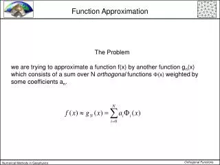
Least-Squares Policy Iteration (Lagoudakis and Parr, 2003) • Linear architecture: • is learned so as to optimally approximate Bellman equation in the least-squares sense • # of parameters is only : • LSPI works well if we choose appropriate • Question: How to choose ? : fixed basis functions : parameters : # of basis functions
Popular Choice: Gaussian Kernel (GK) • Smooth • Gaussian tail goes over partitions Partitions : Euclidean distance : Centre state
Approximated Value Function by GK • Values around the partitions are not approximated well. Optimal value function Approximated by GK Log scale 20 randomly located Gaussians
Policy Obtained by GK • GK provides an undesired policy around the partition. Optimal policy GK-based policy
Aim of This Research • Gaussian tails go over the partition. • Not suited for approximating discontinuous value functions. We propose new Gaussian kernel to overcome this problem.
State Space as a Graph • Ordinary Gaussian uses Euclidean distance. • Euclidean distance does not incorporate state space structure, so tail problems occur. • We represent state space structure by a graph, and use it for defining Gaussian kernels. (Mahadevan, ICML 2005)
Geodesic Gaussian Kernels • Natural distance on graph is shortest path. • We use shortest path in Gaussian function. • We call this kernel geodesic Gaussian. • SP can be efficiently computed by Dijkstra. Shortest path Euclidean distance
Example of Kernels • Tails do not go across the partition. • Values smoothly decrease along the maze. GeodesicGaussian Ordinary Gaussian
Comparison of Value Functions Optimal Ordinary Gaussian Geodesic Gaussian • Values near the partition are well approximated. • Discontinuity across the partition is preserved.
Comparison of Policies Ordinary Gaussian GeodesicGaussian • GGKs provide good policies near the partition.
Experimental Result Average over 100 runs • Ordinary Gaussian: tail problem • Geodesic Gaussian: no tail problem Geodesic Fraction of optimal states Ordinary Number of kernels
Robot Arm Reaching 2-DOF robot arm • Task: move the end effector to reach the object State space 180 Object End effector Obstacle Joint 2 (degree) 0 Joint 2 Joint 1 Reward: +1 reach the object 0 otherwise -180 -100 0 100 Joint 1 (degree)
Robot Arm Reaching Successfully avoids the obstacle and can reach the object. Ordinary Gaussian Geodesic Gaussian Moves directly towards the objectwithout avoiding the obstacle.
Khepera Robot Navigation • Khepera has 8 IR sensors measuring the distance to obstacles. • Task: explore unknown maze without collision Reward: +1 (forward) -2 (collision) 0 (others) Sensor value: 0 - 1030
State Space and Graph Discretize 8D state space by self-organizing map. 2D visualization Partitions
Khepera Robot Navigation When facing obstacle, goes backward (and goes forward again). Ordinary Gaussian Geodesic Gaussian When facing obstacle, makes a turn (and go forward).
Experimental Results Average over 30 runs Geodesic Ordinary • Geodesic outperforms ordinary Gaussian.
Conclusion • Value function approximation: good basis function needed • Ordinary Gaussian kernel: tail goes over discontinuities • Geodesic Gaussian kernel: smooth along the state space • Through the experiments, we showed geodesic Gaussian is promising in high-dimensional continuous problems!