Download
1 / 16
160 likes | 299 Vues
Internal modes of the ocean circulation on decadal to centennial time scales and their mechanism. Thierry Huck , Olivier Arzel , Alain Colin de Verdière Laboratoire de Physique des Océans, Brest, France http://www.ifremer.fr/lpo/thuck/

E N D
Internal modes of the ocean circulation on decadal to centennial time scales and their mechanism Thierry Huck, Olivier Arzel, Alain Colin de Verdière Laboratoire de Physique des Océans, Brest, France http://www.ifremer.fr/lpo/thuck/ • Outline: process studies with idealized ocean and atmosphere models • two different mechanisms for interdecadal variability of the ocean thermohaline circulation under constant flux and mixed surface boundary conditions • which one is relevant with more realistic atmospheric coupling?
Introduction • Variability in the climate system • "external" forcing (solar volcanic anthropogenic) • coupled ocean-atmosphere modes (ENSO) • atmospheric modes (NAO) • internal ocean modes, unstable or damped (and sustained by atmospheric synoptic noise) • + modes involving feedbacks with snow, ice, biosphere... • Aim : exhibit internal modes of the ocean circulation, and understand their mechanism and robustness. • Methods • - nonlinear integrations under prescribed forcing (unstable) • - nonlinear integrations with stochastic forcing (weakly damped) • - linear stability analysis exhibit all modes
Interdecadal ocean variability Several ocean models have shown variability on interdecadal time scales under different types of forcing: - mixed boundary conditions (Weaver and Sarachik 1991, Weaver et al. 1991, 1993) - constant fluxes of heat (Greatbatch and Zhang 1995, Huck et al. 1999, te Raa and Dijkstra 2002) or freshwater (Huang and Chou 1994) Several mechanism have been proposed: advective, boundary waves, large scale ‘generalized’ baroclinic instability • Are all these interdecadal oscillations similar, based on a single mechanism? what is it? • How do they survive with more realistic configurations and atmospheric coupling?
The ocean model • 3D ‘large-scale’ ocean model • - planetary geostrophic dynamics • flat bottom • one-hemisphere configuration • - linear equation of state • RTRS: relaxation of both surface temperature and salinity • steady state • FTFS: diagnosed surface fluxes of heat and salt, prescribed • 57 yr oscillation • RTFS: mixed boundary conditions • 19 yr oscillation after large shift • RT FT: same for temperature only Linear stability analysis • unstable oscillation under FTFS&FT • unstable real mode under RTFS
The ocean mean state Meridional overturning (Sv) and zonally averaged temperature (ºC) Surface heat flux (W/m2) and convection depth (m) FTFS (constant flux) RTFS (mixed)
Anomalies time evolution FTFS (flux): cyclonic recirculation in north-west corner RTFS (mixed): eastward propagation SST (color, K) and SSS (contour, psu) anomalies during half a period
Temperature or salinity? Horizontal basin-averaged perturbation density variance as a function of depth in terms of temperature and salinity _____ _____ _______ σT2=<α2T’2> ; σS2=<β2S’2> ; σTS2=-2<αβT’2S’2> FTFS (flux): temperature RTFS (mixed): salinity
Vertical structure of the perturbations • Phase diagram of temperature and salinity anomalies in the most unstable region for each experiment: • vertical phase lag under flux bc • dipolar structure in temperature under mixed bc FTFS (flux): 49ºN-10ºE RTFS (mixed): 59ºN-39ºE
Density variance budget Driving term for density variance (source): FTFS (flux): RTFS (mixed):
Summary • Interdecadal oscillations under constant flux and mixed boundary conditions have two different mechanisms • which one (if any) is relevant to more realistic atmospheric coupling?
Coupling with an axisymmetric atmospheric model 2D atmospheric model: - primitive equations with full hydrological cycle - parameterizations for meridional eddy transport of momentum, heat and moisture (Yao and Stone 1987, Stone and Yao 1990) - cumulus convection (Manabe et al. 1965) Coupled model climatology with symmetric ocean: zonally-averaged circulation in the atmosphere (megaton/s) and ocean (Sv)
Weakly damped interdecadal variability Maximum meridional overturning streamfunction (Sv) in the Northern hemisphere for the coupled model, and for the stand-alone ocean model forced by combinations of constant surface fluxes of heat, freshwater and momentum • The oscillation mechanism lies in the ocean, the atmosphere surface heat flux feedback damps the variability
Same mechanism as the ”thermal” mode Ocean surface density anomalies (10-3 kg m-3) over an oscillation Driving term for the ocean density variance:
Asymmetric configuration with ACC • ocean with periodic channel 77ºS-60ºS • 22 yr oscillation • Ocean surface density variance (103 kg2/m6), superposed on mean surface current 0-250m • variability restricted to northern hemisphere
Conclusions • These 'simple' oscillations provide prototypes to understand physical mechanisms of oscillations in more complex (coupled) models • The density variance budget provides a method to identify different sources of variability, that can be applied to realistic and coupled models • These mechanisms found in idealized geometry need to be tested in more realistic configurations (see poster by Sévellec et al. about optimal surface salinity perturbations) • Unfortunately, interdecadal variability in state-of-the-art coupled models seems most often due to coupled mechanisms: what happens to these internal ocean modes?
Internal modes of the thermohaline circulation and their mechanism Tools: density variance budget, linear stability analysis, bifurcation diagrams, dynamical system theory