Download
1 / 14
140 likes | 265 Vues
A functional form for the spatial distribution of aftershocks. Karen Felzer USGS Pasadena. Summary. Aftershock density decays with distance, r , from the mainshock surface as r -n where n =1.3 -- 2.5 and may vary for different mainshocks .

E N D
A functional form for the spatial distribution of aftershocks Karen Felzer USGS Pasadena
Summary • Aftershock density decays with distance, r, from the mainshock surface as r-nwhere n=1.3 -- 2.5 and may vary for different mainshocks. • This decay holds out to distances of at least 50-100 km for mainshocks of all magnitudes. • The azimuthal distribution of aftershocks appears to vary according to receiver fault locations (Powers, 2009) and mainshock propagation direction (Kilb et al. 2000).
Advantages & disadvantages of using small mainshocks • Mainshocks can be treated as point sources at most distances – no worries about main shock fault plane location and complexity. • Many aftershock sequences are stacked to see the signal. The use of many sequences => results provide a good regional average. • The use of many sequences also drives up inclusion of background earthquakes => may make the decay appear too slow.
Small mainshocks and the background earthquake problem Observe aftershocks for 60 minutes after mainshock Observations include 60 minutes of background earthquakes Big Mainshock Observe aftershocks for 60 minutes after mainshocks Observations include 600 minutes of background earthquakes 10 small main shocks
Best fit aftershock decay for M 1—2 main shocks in Northern California from 1-10 km: Density ~ r-1.3 8656 M 1—2 Northern California mainshocks from the NCSN catalog, not preceded by larger event for 3 days/200 km
Best fit aftershock decay for M 2—4 main shocks in Southern California from 1-100 km: Density ~ r-1.4 M ≥2 Aftershocks taken from the first 5 minutes after each mainshock From Felzer and Brodsky (2006)
Advantages and disadvantages of using bigmain shocks • Main shocks can be inspected individually, decreasing interference from background seismicity. • Results may be specific to a particular location or event. • Unknown complexity of the main shock fault plane and incomplete catalogs may cause error.
Best fit aftershock decay for M ~ 5 Anza earthquakes, 4-40 km: Density ~ r-1.8 68 M≥0.5 aftershocks from 4-40 km 49 M≥0.5 aftershocks from 4-40 km From Felzer and Kilb(2009)
M 7.2 El Mayor-Cucapah earthquake: Density ~ r-2.0 Aftershocks to the north clearly concentrated on the Elsinore and San Jacinto fault zones
Similar work by other authors Marsan and Lengline(2010) M 3—6 main shocks, hard work to decrease background seismicity interference Density ~ r-1.7--r-2.1
Conclusions • Aftershock density decays with distance, r, from the mainshock surface as r-nwhere n ~ 1.3 – 2, probably 1.8--2?? • This decay is seen out to distances of 50—100 km for mainshocks as small as M 1.0. • The azimuthal distribution of aftershocks may be influenced by existing faults.
More to come about big mainshocks in my next talk! Hector Mine earthquake scarp