Chapter 3 The Demand for Labor
360 likes | 617 Vues
Chapter 3 The Demand for Labor. Outline. Profit Maximization Short-Run Demand (in competitive markets) Long-Run Demand Labor Demand with non competitive product market The Effects of Payroll Taxation The Effects of Wage Subsidies Monopsony. Profit Maximization.

Chapter 3 The Demand for Labor
E N D
Presentation Transcript
Chapter 3 The Demand for Labor
Outline • Profit Maximization • Short-Run Demand (in competitive markets) • Long-Run Demand • Labor Demand with non competitive product market • The Effects of Payroll Taxation • The Effects of Wage Subsidies • Monopsony
Profit Maximization • Microeconomic problem: Maximize Profits (Revenues minus costs) by optimally choosing output • …but output can be changed by varying inputs • 2 key factors of production (Labor and Capital) • Change in one input, holding other input constant • Rule of thumb: • If net profit generated by an extra input is positive, then add unit • If net profit generated by an extra input is negative, then reduce unit • If net profit generated by extra input is zero, no further changes are required
Marginal Products & more • Marginal Product MPL: change in output (ΔQ) produced by a change in labor, holding capital constant MPL= ΔQ/ ΔL (constant capital) • Marginal Revenue MR: • If product market is competitive (firm is price taker): MR=P • If firm has market power in the good market: MR<P • Marginal Revenue Product MRPL: • If product market is competitive MRPL=MPL*P • If firm has market power : MRPL=MPL*MR
Marginal Product: Few Examples • Blue Collar Worker in Car Industry: • P: price of cars • MP: number of extra cars produced • Bocconi Professor • P: Tuition fee paid by students • MP: number of additional courses taught • Soccer Player • P: ticket price at the stadium (or pay per view) • MP: number of additional seats sold
Marginal Expenses: Costs • If the firm compets in the factor market, • W: wage rate is the unit cost of (homogenous) labor. Cost of hiring an hour of worker • C: the price of capital • MEL=W
Short Run Demand for Labor • Short-Run: period over which capital can not be varied • A Key Assumption: Declining MPL (the law of diminishing return) • Use Rule of Thumb: expand employment as long as MRPL>MEL, up to MRPL=MEL
Figure 3.1 Demand for Labor in the Short Run (Real Wage)
…short run labour demand • Labour Demand in terms of real wages (wages measured in terms of output): • The demand for labour in the short-run is always the downward sloping segment of MPL • (if MPL, increasing, then employment should be expanded….) • Market Demand: summation of the labour demanded by all firms in a particular market at ech level of the real wages
Figure 3.2 Demand for Labor in the Short Run (Money Wage)
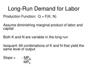
Long-Run Labour Demand • MRPL=W; in competitive mkts: MPL*P=W • MRPK=C; in competitive mkts: MPK*P=W • This can be written as • P=W/ MPL and P=C/ MPk so that • W/ MPL= =C/ MPk • The marginal cost of producing an added unit of output using labour is equal to the marginal cost of producing an added unit of output using capital
Effect of Increase in the Price of One Input (k) on Demand for Another Input ( j ), Where Inputs Are Substitutes in Production Figure 3.3
Labour Demand if Product Market is Non Competitive • A Monopolist trying to maximize profits with a competitive labour market • MRPL=MR*MPL=W • Wage rate paid by monopolists are not necessarily different from competitive markets, even though employment level is..
Monopsony in the Labour Market • Only one firm is the buyer of labour in the market • E.g. large firms in small town (coal mining town) • Rathen than begin wage taker, monopsonit face upward sloping labour supply • Competitive Firm: the cost of hiring an extra worker (from 1 to 2) is the wage rate • Monopsonist: When hiring the second worker, the firm must pay a higher wage to all workers
Monopsonist • Upward sloping Supply: • If it hires 2 worker the wage rate is $7 per worker (total $14) • If it hires 3rd workers the wage rate is $7.5 per worker • For a Monopsonist hiring the third worker costs $7.5*3=$22.5; but $22.5-$14=$8.5! • Key Aspect: marginal expense of labor exceeds the wage: MEL>W • Profit Maximization: MRPL=MEL
Figure 3.4 The Effects of Monopsony
The Monopsonist’s Short-Run Response to a Leftward Shift in Labor Supply: Employment Falls and Wage Increases Figure 3.5
Minimum Wage Effects under Monopsony: Both Wages and Employment Can Increase in the Short Run Figure 3.6
The Effects of Employer Payroll Taxes • Who Bears the burden of a payroll tax? • Let us consider a social insurance tax paid by the employer. • The party making the payment is not necessarily the one that bears the burden of the tax! • With Payroll Taxes, Employer wage costs are larger than what employees received (a tax wedge)
A Tax Wedge • Suppose tax is fixed amount X per hour, rathern than proportional • Plot Labor demand against wage that employees receive • Without tax the wage employer pay is the same as wage employees receive • After the tax is imposed, the wage cost> wage received • ….the labor demand shifts down, with a fixed shift equal to X
The Market Demand Curve and Effects of an Employer-Financed Payroll Tax Figure 3.7
Burden of payroll tax • New equilibrium has lower employment and lower wage after tax wage • Employees bear a burden in the form of lower wage rates and lower employment • ….but the wage does not fall by the full amount of the tax, so that employers also bear some of the tax • …..unless labor supply is perfectly vertical.
Figure 3.8 Payroll Tax with a Vertical Supply Curve
What the data say? • How do individuals respond to payroll taxes? • Is employment reduced? • How is the slope of the labor supply in real life labor markets? • ….difficult to say, but most empirical studies tend to find that in the long run labor supply (for prime age males) is vertical, and workers bear the entire burden of the tax • In other words, the tax transaltes into lower wages with little effects on total labor costs
Are Payroll Taxes Responsible for European Unemployment? • Various social programs: social security contributions, health, unemployment benefits….. • …are financed by payroll taxes • Facts: • Payroll taxes are a large part of earnings • They are generally larger in Europe than in the US • So they may be potentially responsible for unemployment • Indeed, these taxes raised as unemployed increased. • But overall evidence is mixed (micro evidence versus macro facts) • The case of Denmark particularly interesting
Microeconomics Overview • Isoquants: combination of labor and capital that produce some level of output • …they have negative slopes (labor and capital are substitutes) • …they are convex (step slope ay low labor and almost flat when labor is high) • MRTS (Marginal Rate of Technical Substitution) • MRTS=(K/ L)|Q fixed
Figure 3A.1 A Production Function
Demand for Labor Short-Run • Capital is fixed in the short run • Slope of the isoquant at a given K decreases as output grows • ….each successive labor hour hired generates progressively smaller increments in output (by assumption, see labels isoquants)
Figure 3A.2 The Decline Marginal Productivity of Labor
Cost Minimization in the Production of Q* (Wage = $10 per Hour; Price of a Unit of Capital = $20) Figure 3A.3
Cost Minimization in the Production of Q* (Wage + $20 per Hour; Price of a Unit of Capital + $20) Figure 3A.4
Figure 3A.5 The Substitution and Scale Effects of a Wage Increase