Demystifying Census Data
Demystifying Census Data. Legislative Research Librarians September 18, 2013 Boise, Idaho. Agenda. Demographic programs Census geography Race and ethnicity Accessing the data Tips: Presenting the data Topic-driven searches Resources Summary. Demographic Programs. 2010 Census

Demystifying Census Data
E N D
Presentation Transcript
DemystifyingCensus Data Legislative Research Librarians September 18, 2013 Boise, Idaho
Agenda • Demographic programs • Census geography • Race and ethnicity • Accessing the data • Tips: Presenting the data • Topic-driven searches • Resources • Summary
Demographic Programs • 2010 Census • Counts: number of people and housing units • 100% coverage • American Community Survey (ACS) • Estimates demographic, social, economic characteristics of people and housing stock • Characteristics: how people live • Sample of 2.5% of U.S. households every year
Questionnaire Topics2010 Decennial Census (Name) Sex Age Date of birth Ethnicity Race Relationship of people within household Rent / own house (tenure) (Coverage questions)
Census.gov > (footer > About Us column)Census Questionnaires
Questionnaire TopicsAmerican Community Survey (ACS) Items in red were also collected on the 2010 Census
2013 Release DatesACS 2012 Products • 1-year ACS 2012 estimates • September 19 • 3-year ACS 2010-2012 estimates • October 24 • 5-year ACS 2008-2012 estimates • December 5 • To include current state legislative district boundaries
Census.gov > (footer > People & Households column)ACS Questionnaires
American Community Survey In a Nutshell • Strengths • Data are current • Rich topical detail • Challenges • Reliability issues due to sample size • Small areas • Small population groups • Data user must consider margin of error (MOE) when using ACS estimates
ACS Updates and Improvements Sample Size Increase • Sample expanded from 2.9 million to 3.54 million addresses per year • Begun during 2011 data collection • Mail out -- June 2011 • CATI (Computer-Assisted Telephone Interview) -- July 2011 • CAPI (Computer-Assisted Personal Interview) -- August 2011
ACS Updates and Improvements Reallocation of Sample • Objective: Improve the reliability of the estimates for small areas • Increased sampling rates for small tracts and governmental units • Slightly decreased sampling rates in larger tracts • Begun in January 2011
ACS Updates and Improvements: New QuestionsComputer Ownership / Internet Usage
ACS Updates and ImprovementsInternet Response Option • Ongoing digital transformation • 61st U.S. Census Bureau survey with Internet response option • Households in sample receive letter with login instructions to secure website • Participants have the ability to review responses • Assistance available to respondents • Advantages • More convenient for respondents • More cost-effective • Secure and confidential
Census Geography Hierarchy (with 2010 Statistical Area Criteria) Revised 02-19-13 Central axis describes a nesting relationship Block Groups • Types of Place • Cities and towns -- incorporated • Census Designated Places (CDPs): • - - Unincorporated; no size threshold • - - Separate and distinct from city/town • - - Redefined each census • 600 to 3,000 population • 240 to 1,200 housing units • Blocksnot defined by population • Lowest geographic level for data • Census Tracts • 1,200 to 8,000 population (optimum 4,000) • 480 to 3,200 housing units Block level data only for Decennial Census
Small Area Geography Hierarchy • Block number: Blocks have 4-digit numbers – their block group number (“3” in this illustration) is the first digit. • Block group number: Always a single digit (1 to 9). • Census tract number: A decimal indicates that a census tract has been split, usually because it has exceeded the optimum size (housing units or population). This enables comparability from census to census. • Decennial Census: Lowest level of geography on American FactFinder (AFF) - - block. • American Community Survey: Lowest level of geography on AFF - - census tract; on the FTP (download) site - - block group.
2010 Census (Boise city, ID)Tract Reference Maps(block maps also available) • Homepage > Geography tab > Maps and Data > Reference Maps > Census Reference Maps > Census Tract Maps (2010) > place (select state) GO > (select county) > click hyperlink for place name > if more than one map sheet, open 000.pdf (index map) to determine map sheet number (or inset letter) > back out > select map sheet (or inset)
2010 Census Ethnicity Question (asked since 1970) 2010 Census Race Question (asked since 1790)
Quick Data Tools • Quick Facts • Interactive Map • Population Finder
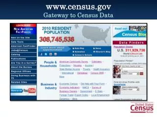
Census Homepage: census.gov Data tab: Easy Stats
Census Homepage: census.gov Data tab: American FactFinder
factfinder2.census.govAmerican FactFinder (AFF) Community Facts tab
Assistance with American FactFinder • Click Help(AFF mainpage, top right) • Online User Guide • Virtual Tour • Community Facts • Guided Search • Advanced Search • Download Options • Using Data • Tables • Maps • Narrative Profiles • Tutorials • Glossary
factfinder2.census.govAmerican FactFinder (AFF) Guided Search tab
AFF Guided Search User answers prompts, then clicks “Next” or a numbered arrow to proceed -- arrows 1 through 4 may be selected in any order
factfinder2.census.govAmerican FactFinder (AFF) Advanced Search tab
Advanced Search page Filter bars facilitate searches. Object is to select filters, such as Topics, to refine search. All filters will appear in the Your Selections box to be applied to the final table selection. See next slide for Topics sub-categories
Four Tips for Using Census Data • Use the most appropriate source • Understand census jargon • Use census data to draw comparisons between two different geographies or two different population groups • Use census data to look at changes over time
Census Data Profiles • Four fact sheets on the social, economic, housing, and demographic characteristics of different geographic areas • More than 450 characteristics for an area, depicting how people live • Excellent starting point for research • Data profiles may help identify a problem • May need a different table with more specific information to quantify a problem
Data in a Grant Proposal • Present data that demonstrates a need • Reflect funding agency priorities • If you are serving a small population, provide census tract data • Show data and derived measures as reference points • Example: 3,000 families below poverty, or 15%
Provide Comparisons • Over time (2000, 2010) • Demonstrate emerging issues affecting your target population • Be mindful of boundary changes • Compare subset data to larger group • State to national • City/town to county or state • Census tract to other tracts or to city/county
Two Censuses: Power of Comparisons Percent change equation: New minus Old divided by Old multiplied by 100 (fictitious geography)
Charts and GraphsGood Data Visualization • Reduces “cognitive load” • Enables reader to understand relationships quickly and clearly • Is self-explanatory • Narrative can provide background • “The chart on the next page illustrates increases in the American Indian population over the past 30 years”
Race Categories: Alone or Combo • Choices for data user to make: • Race Alone (smaller number), or • Race Alone or in Combination
Presenting the DataTips • Show both data and derived measures • Example: 3,000 families, or 15%, are living below the poverty level • Note the “universe” for the table • Example: “Population for whom poverty status is determined” • Two data points do not define a “trend”
Derived Measures* *A unit that is determined by combining one or more measurements • Mean = average • Median • Percent • Rate The ACS generally does a better job estimating percentages, rate, means, and medians than it does totals
Income EstimatesMean = Average Salaries of nine workers at the World Wide Widget Company: The CEO makes $100,000 per year, Two managers make $50,000 per year, Four factory workers make $15,000 each per year, and Two trainees make $9,000 each per year. Add $100,000 + $50,000 + $50,000 + $15,000 + $15,000 + $15,000 + $15,000 + $9,000 + $9,000, which gives you $278,000. Then you divide that total by 9 -- the number of values or workers in the set of data This gives you the mean or average, which is $30,889 Be careful! Only three of the nine workers at WWW Co. make that much money, and the other six workers don’t even make half the average salary. So what statistic should you use when you want to give some idea of what the average worker at WWW Co. is earning? Let’s look at the median.
Income EstimatesMedian (preferred) When you speak about the average worker or average household, you really want a statistic that tells you something about the worker or the household in the middle. Again, this statistic is easy to determine because the median literally is the value in the middle. Just line up the values in your set of data, from largest to smallest. The one in the dead-center is your median. Below are the nine WWW Co. workers’ salaries: $100,000 $50,000 $50,000 $15,000 $15,000 $15,000 $15,000 $9,000 $9,000 The one halfway down the list, the fifth value, is $15,000. That’s the median. If you have an even number of values, split the difference between the two in the middle. Comparing the mean ($30,889) to the median ($15,000) gives you an idea how widely the values in your dataset are spread apart.