Body frame
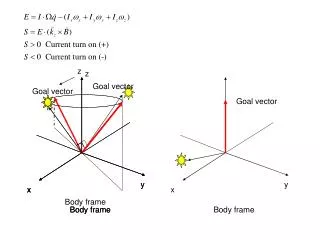
z. z. Goal vector. Goal vector. x. x. y. x. Body frame. Body frame. Body frame. Goal vector. y. y. x. Body frame. Sun normal: Spin mode (assume omega x= omega y=0). Rad/sec. 4 rpm. Sun elevation near 90 degree (random). omega x, omega y ==0

Body frame
E N D
Presentation Transcript
z z Goal vector Goal vector x x y x Body frame Body frame Body frame Goal vector y y x Body frame
Sun normal: Spin mode (assume omega x= omega y=0) Rad/sec 4 rpm Sun elevation near 90 degree (random) omega x, omega y =\=0 If we want to eliminate them, we need to estimate them.
Sun normal: precession mode (assume omega x= omega y=0) Elevation=0 (not ecliptic normal) Not good for initial conditions with high elevation
Ecliptic plane The sun ECI vector The sun ECI vector
High elevation The sun ECI vector
One strategy: only using one side controller (elevation >0 or elevation <0) Open controller Open controller elevation elevation
Omega change Because we only use one coil in z axis, the effects to the spin rate are small 4 rpm omega x, omega y
Conclusion: 1 The storage of battery for the ACS is ok (0.7 w for each “turn on” operation ) 2 test other initial conditions for sun normal mode Issue: 1 need to figure out what happen in the high elevation 2 PIC operation temperature -40 oC~ 85 oC 3 If there are two fixed vectors in the ECI frame, is it possible to know the angular velocities of the three dimension (without any information from the ground )? t1 t2 3.75 A hour at 8 volt sun B field sun B field In the view of the body In the view of the body
z z Goal vector Goal vector x x y x Body frame Body frame Body frame Goal vector y y x Body frame
z Goal vector x x Body frame Body frame based on the same fixed vector in ECI z Goal vector is fixed Y x ECI frame If there exists omega x or omega y, the goal vector is no longer fixed in the ECI frame
Solver problem Time frame =0.01 Time frame =0.1 Time frame =0.01 Time frame =0.1
Different model structure may produce the errors ! Give the Sun ECI initial condition Give the initial attitude Elevation of the sun in the body frame Give the Sun ECI initial condition Due to omega x ,omega y
Mass: 10e-9 kg Moment of inertia: 10e-7 kgm^2 Equator plane Revolute around local x Revolute around local y Revolute around local z ground
ECI Equator plane Revolute around local x,y,z And allow slide in x,y,z direction ground
Omega x,y,z 4 rpm Elevation=0 Sun normal :spin up detumble Sun normal: precession
elevation Precession Sun normal precession Sun normal precession Deviation of the attitude (ecliptic normal)
Assume: local b field not change much bx bz Z by x y Rotation matrix: Y(90 degree)Z(180 degree)
simulation Local b field ECEF local b field body frame local magnetometer frame rotation matrix and normalized module In PIC ACS module
Z+ Y+ elevation X+ Power from each solar panel (total six panels) 1: with 10 degree constraints for each panel 2: the energy is proportional to the area 3: 15% efficiency for each panel 4: also including the power from the albedo 5 assume in each panel, the power is uniform 6 the area of the solar panel, right now: (10x10 cm) meter square 7 assume the storage: 3.75 A hour at 8 volt=108000 =10o X- Y- Z-
“for the (-X) side, the magnetic dipole moment is estimated to be 0.87 Am2consuming 6.43 Watts and drawing 0.80 Amperes. The projected values for the (-Z) side [which has not been built yet] are 0.85 Am2 for the magnetic dipole, 8.63 Watts for power and 1.08 Amperes for current.” Assume 10 duty cycle Results: J for every 0.1 second Sun+albedo Error attitude Coil z Coil x
Max PIC energy consumption W=250 mA*4.0V=1W
? 1: W=(125-(-40))/40=4.125w maximum allowed power Dissipation or the chip will melt away. 2: W=(100-80)/40=0.5w <1w
Indirect access values: Receive from Rs232, don’t care which memory the compiler assigned … Transmit through Rs232 With pointers assigning specific address
Int main (){ In the future, replaced by other modules, like sun sensor module, MAG module, etc. Just write to the same memory Data from RS232 Store in the specific memory other work HSK read values from the specific memory ACS reads values from the specific memory Fixed, no change ACS store values to the specific memory (Torque command) other work HSK read values from the specific memory In the future, replaced by toque command module write to the specific memory Data to RS232 }
simulink PIC Another issue: 1:0.7 =real time: simulink
Indirect access values: Receive from Rs232, don’t care which memory the compiler assigned … Transmit through Rs232 With pointers assigning specific address
Protocol design and tasks Data set Begin byte Begin byte Serial data 0 1 2 3 0 1 2 3 ….. ….. data0 data1 Each variable (total 17) is float, each float includes 4 bytes (17x4=68) 1 separate each variable (float->byte) 2 transmit them in the serial port of Simulink 3 receive them in the serial buffer of PIC 4 combine them in the PIC (byte-float)
Structure for parallel testing (run PIC and simulink at the same time, at the same simulink file) Guarantee , the time of switching mode are the same Space Environment, Sensor, CINEMA Guarantee all the initial conditions are the same Serial encode Simulink serial interface Serial decode Serial decode ACS in simulink(c code) ACS in PIC (c code) torque Serial encode Serial encode Simulink serial interface Serial decode Serial decode Coil status Coil status
Experiment results for the controller (new version) simulink PIC
Z+ Y+ elevation X+ Power from each solar panel (total six panels) 1: with 10 degree constraints for each panel 2: the energy is proportional to the area 3: 15% efficiency for each panel 4: also including the power from the albedo 5 assume in each panel, the power is uniform 6 the area of the solar panel, right now: (10x10 cm) meter square (x+-:3, y+-:1, z+-:1) 7 assume the storage: 3.75 A hour at 8 volt=108000 =10o X- Y- Z-
Accumulating energy The day is longer than the night
Ecliptic normal Y+ elevation X+ Z+
Magnetometer sample time: 2 Hz extrapolation Norm of the error in 3 direction
Magnetometer sample time: 5 Hz extrapolation Norm of the error in 3 direction
10Hz 5 Hz
Detumble 2Hz sample time Detumble+spin up Raw edge
Model Predictive Control MPC slides from Prof. Francesco Borrelli
Least square Using one coil Do control only for s>0(spin) s>0 s<0 (spin)
Solution sets MPC—using the information of the future and current B field One coil with fixed duty cycle Two coils with fixed duty cycle Least square—using the current B field with two coils and various duty cycle
Example--- Get the maximum profits from the Banks in 2 years Need the transfer fee from one bank to the other. The interest rates also depend the total saving in each account One coil: BOA, only allowed to put the all of the money in or out Two coils: Citi, BOA, only allowed to put all of the money in one account Least square: : Citi, BOA, allowed to adjust the money in each account. MPC: Citi, BOA allowed to adjust the money in each account and know the interest rates in the future. This method can also consider other situations.
Linearized the nonlinear systems continuous model continuous model discrete model Set the system structure and parameters for the solver k=k+1 Set the translate target set Solver produce the control command Update the current state and insert to the nonlinear system N=N+1
N=0 Initial state N=1 Nonlinear system N=2 N=3 wz K=1 K=2 Translate target set Final target set wy wx
Results: polytope for the feasible region The geometry will update for each k