Fig. 4-1
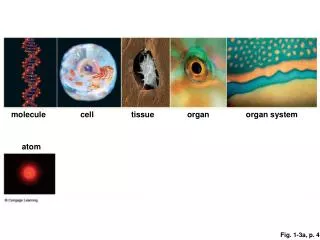
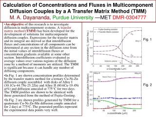
Chapter 4 overview. Fig. 4-1. Genetic recombination : mixing of genes during gametogenesis that produces gametes with combinations of genes that are different from the combinations received from parents. Independent assortment of homologous chromosomes (Anaphase I). Genes on non-
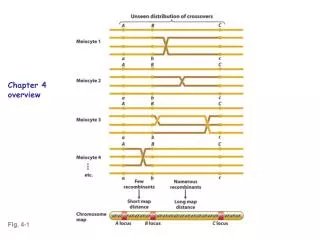

Fig. 4-1
E N D
Presentation Transcript
Chapter 4 overview Fig. 4-1
Genetic recombination: mixing of genes during • gametogenesis that produces gametes with • combinations of genes that are different from • the combinations received from parents. • Independent assortment of homologous • chromosomes (Anaphase I). Genes on non- • homologous chromosomes (unlinked genes) • assort independently.
Using a testcross to distinguish gamete genotypes Fig. 4-7
50% = independent assortment (genes are not linked) Fig. 4-8
Genetic recombination: mixing of genes during • gametogenesis that produces gametes with • combinations of genes that are different from • the combinations received from parents. • Independent assortment of homologous • chromosomes (Anaphase I). Genes on non- • homologous chromosomes (unlinked genes) • assort independently. • Crossing over (recombination among linked • genes)
cis linked: both dominant alleles on the same homolog trans linked: dominant alleles on different homologs Fig. 4-2
Crossing over • Physical exchanges among non-sister chromatids; • visualized cytologically as chiasmata • Typically, several crossing over events occur within • each tetrad in each meiosis (chiasmata physically • hold homologous chromosome together and assure • proper segregation at Anaphase I) p. 115
Crossing over occurs at the four-strand stage (pre-meiotic G2 or very early prophase I) Fig. 4-4
Crossing over can involve 2, 3, or 4 chromatids in a single meiosis Fig. 4-5
Crossing over • Physical exchanges among non-sister chromatids; • visualized cytologically as chiasmata • Typically, several crossing over events occur within • each tetrad in each meiosis (chiasmata physically • hold homologous chromosome together and assure • proper segregation at Anaphase I) • The sites at which crossing over occur are random • The likelihood that a crossover occurs between any • two particular sites (genes) is a function of the • physical distance between those two sites
Crossing over usually affects a minority of chromatids in a collection of meioses – recombinants are typically a minority of products Fig. 4-9
<50% = linked genes Fig. 4-10
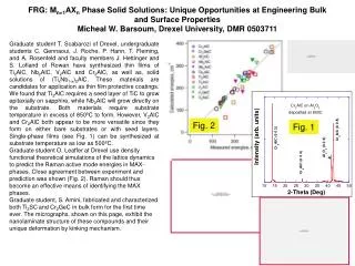
A.H. Sturtevant (1911-3): frequency of crossing over between two genes is a function of their distance apart on the chromosome; created the first genetic map number of recombinants Recombination frequency = total number of progeny One map unit = one centimorgan = 1% recombinants
Rationales: • Crossover events are random • Greater separation, greater likelihood that crossover will occur • Map distance should be sum of smaller intervals • Construct entire chromosome maps by mapping intervals • Linear map correlates with linear chromosome Fig. 4-11
Markers used in trihybrid testcross in Drosophila v = vermilion eyes (red eyes; v+are red-brown) cv = crossveinless (cv+ wings have crossveins) ct = cut wing (ct+ wings have regular margins)
Data from three-point testcross v+/ v cv+/ cv ct+/ ct X v / v cv / cv ct / ct (trihybrid) (tester) Progeny phenotypes v cv+ ct+ 580 v+ cv ct 592 v cv ct+ 45 v+ cv+ ct 40 v cv ct 89 v+ cv+ ct+ 94 v cv+ ct 3 v+ cv ct+ 5 1448
Steps in solving three-point testcross problem • Anticipate and identify eight types of products (23) • Identify pairs of reciprocal products
Data from three-point testcross v+/ v cv+/ cv ct+/ ct X v / v cv / cv ct / ct (trihybrid) (tester) Progeny phenotypes v cv+ ct+ 580 v+ cv ct 592 v cv ct+ 45 v+ cv+ ct 40 v cv ct 89 v+ cv+ ct+ 94 v cv+ ct 3 v+ cv ct+ 5 1448
Steps in solving three-point testcross problem • Anticipate and identify eight types of products (23) • Identify pairs of reciprocal products • Identify parental types as the most frequent pair of • products • Identify double crossover products as least frequent • pair of products
Data from three-point testcross v+/ v cv+/ cv ct+/ ct X v / v cv / cv ct / ct (trihybrid) (tester) Progeny phenotypes v cv+ ct+ 580 v+ cv ct 592 v cv ct+ 45 v+ cv+ ct 40 v cv ct 89 v+ cv+ ct+ 94 v cv+ ct 3 v+ cv ct+ 5 1448 Parental types - nco sco sco dco
Steps in solving three-point testcross problem • Anticipate and identify eight types of products (23) • Identify pairs of reciprocal products • Identify parental types as the most frequent pair of • products • Identify double crossover products as least frequent • pair of products • Compare the parental and double crossover products • to deduce the order of the three gene loci
Fig. 4-12 In dco products, the central marker is displaced relative to the parental types
Steps in solving three-point testcross problem • Anticipate and identify eight types of products (23) • Identify pairs of reciprocal products • Identify parental types as the most frequent pair of • products • Identify double crossover products as least frequent • pair of products • Compare the parental and double crossover products • to deduce the order of the three gene loci • Compute map distances by breaking down the • results for each interval
Fig. 4-12 85 + 8 1448 (0.064) 183 + 8 1448 (0.132) RF =
Fig. 4-12 85 + 8 1448 (0.064) 183 + 8 1448 (0.132) RF = 13.2 m.u. 6.4 m.u. v ct cv
Interference: crossing over in one region interferes with simultaneous crossing over in adjacent regions Expected frequency of dco = product of frequency crossovers in two regions 0.132 X 0.064 = 0.0084 0.084 X 1448 = 12 expected (if two sco are independent events)
Interference: crossing over in one region interferes with simultaneous crossing over in adjacent regions Expected frequency of dco = product of frequency crossovers in two regions 0.132 X 0.064 = 0.0084 0.084 X 1448 = 12 expected (if two sco are independent events) Coefficient of coincidence = observed dco / expected dco 8 / 12 = 0.667 Interference = 1 – coefficient of coincidence 1 – 0.667 = 0.333
Fig. 4-14 Tomato karyotype (n=12)
Tomato linkage map (1952) Fig. 4-14
Typical phenotypic ratios for a variety of crosses (complete allele dominance) p. 136