Download
1 / 73
740 likes | 1.19k Vues
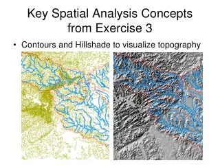
Key Spatial Analysis Concepts from Exercise 3 . Contours and Hillshade to visualize topography. Zonal Average of Raster over Subwatershed. Subwatershed Precipitation by Thiessen Polygons. Thiessen Polygons Feature to Raster ( Precip field) Zonal Statistics (Mean) Join

E N D
Key Spatial Analysis Concepts from Exercise 3 • Contours and Hillshade to visualize topography
Subwatershed Precipitation by Thiessen Polygons • Thiessen Polygons • Feature to Raster (Precip field) • Zonal Statistics (Mean) • Join • Export to DBF (Excel)
Subwatershed Precipitation by Interpolation • Kriging (on Precip field) • Zonal Statistics (Mean) • Join • Export
Runoff Coefficients • Interpolated precip for each subwatershed • Convert to volume, P • Sum over upstream subwatersheds • Runoff volume, Q • Ratio of Q/P
Digital Elevation Model Based Watershed and Stream Network Delineation • Conceptual Basis • Eight direction pour point model (D8) • Flow accumulation • Pit removal and DEM reconditioning • Stream delineation • Catchment and watershed delineation • Geomorphology, topographic texture and drainage density • Generalized and objective stream network delineation
Readings • Arc Hydro Chapter 4 • At http://help.arcgis.com, start from “An overview of the Hydrology tools” http://help.arcgis.com/en/arcgisdesktop/10.0/help/009z/009z0000004w000000.htm to end of Hydrologic analysis sample applications
Conceptual Basis • Based on an information model for the topographic representation of downslope flow derived from a DEM • Enriches the information content of digital elevation data. • Sink removal • Flow field derivation • Calculating of flow based derivative surfaces • Delineation of channels and subwatersheds
Duality between Terrain and Drainage Network • Flowing water erodes landscape and carries away sediment sculpting the topography • Topography defines drainage direction on the landscape and resultant runoff and streamflow accumulation processes
The terrain flow information model for deriving channels, watersheds, and flow related terrain information. Watersheds are the most basic hydrologic landscape elements Pit Removal (Filling) Raw DEM Channels, Watersheds, Flow Related Terrain Information Flow Field
DEM Elevations 720 720 Contours 740 720 700 680 740 720 700 680
80 80 74 74 63 63 69 69 67 67 56 56 60 60 52 52 48 48 Hydrologic Slope - Direction of Steepest Descent 30 30 Slope: ArcHydro Page 70
32 64 128 16 1 8 4 2 Eight Direction Pour Point Model ESRI Direction encoding ArcHydro Page 69
2 2 4 4 8 1 2 4 8 4 32 64 128 4 1 2 4 8 16 1 2 4 4 4 4 8 4 2 1 2 1 4 16 Flow Direction Grid ArcHydro Page 71
32 64 128 16 1 8 4 2 Flow Direction Grid
Grid Network ArcHydro Page 71
Flow Accumulation Grid. Area draining in to a grid cell 0 0 0 0 0 0 0 0 0 0 0 2 2 2 0 2 2 0 0 2 0 1 0 0 10 0 0 1 0 10 1 0 0 0 14 0 1 0 0 14 1 0 4 1 19 4 1 0 1 19 Link to Grid calculator ArcHydro Page 72
Stream Network for 10 cell Threshold Drainage Area Flow Accumulation > 10 Cell Threshold 0 0 0 0 0 0 0 0 0 0 2 2 0 0 2 0 2 2 2 0 0 0 1 0 0 1 10 0 0 10 0 1 0 0 1 0 0 14 0 14 4 1 0 1 1 0 4 1 19 19
1 1 1 1 1 1 3 3 3 1 1 2 1 1 11 2 1 1 1 15 2 1 5 2 20 TauDEM contributing area convention. 1 1 1 1 1 3 3 1 1 3 1 1 2 1 11 1 2 1 1 15 5 2 1 2 25 The area draining each grid cell includes the grid cell itself.
Streams with 200 cell Threshold(>18 hectares or 13.5 acres drainage area)
Watershed andDrainage PathsDelineated from 30m DEM Automated method is more consistent than hand delineation
The Pit Removal Problem • DEM creation results in artificial pits in the landscape • A pit is a set of one or more cells which has no downstream cells around it • Unless these pits are removed they become sinks and isolate portions of the watershed • Pit removal is first thing done with a DEM
Pit Filling Increase elevation to the pour point elevation until the pit drains to a neighbor
Parallel Approach • Improved runtime efficiency • Capability to run larger problems • Row oriented slices • Each process includes one buffer row on either side • Each process does not change buffer row
Pit Removal: Planchon Fill Algorithm 2nd Pass 1st Pass Initialization Planchon, O., and F. Darboux (2001), A fast, simple and versatile algorithm to fill the depressions of digital elevation models, Catena(46), 159-176.
Communicate Parallel Scheme D denotes the original elevation. P denotes the pit filled elevation. n denotes lowest neighboring elevation i denotes the cell being evaluated
Improved runtime efficiency Parallel Pit Remove timing for NEDB test dataset (14849 x 27174 cells 1.6 GB). 8 processor PC Dual quad-core Xeon E5405 2.0GHz PC with 16GB RAM 128 processor cluster 16 diskless Dell SC1435 compute nodes, each with 2.0GHz dual quad-core AMD Opteron 2350 processors with 8GB RAM
The challenge of increasing Digital Elevation Model (DEM) resolution 1980’s DMA 90 m 102 cells/km2 1990’s USGS DEM 30 m 103 cells/km2 2000’s NED 10-30 m 104 cells/km2 2010’s LIDAR ~1 m 106 cells/km2
Capabilities Summary 11 GB 6 GB 4 GB 1.6 GB 0.22 GB Single GeoTIFF file size limit 4GB At 10 m grid cell size
Carving Lower elevation of neighbor along a predefined drainage path until the pit drains to the outlet point
Filling Minimizing Alterations Carving
“Burning In” the Streams Take a mapped stream network and a DEM Make a grid of the streams Raise the off-stream DEM cells by an arbitrary elevation increment Produces "burned in" DEM streams = mapped streams = +
AGREE Elevation Grid Modification Methodology – DEM Reconditioning
Stream Segments 201 172 202 203 206 204 Each link has a unique identifying number 209 ArcHydro Page 74
Vectorized Streams Linked Using Grid Code to Cell Equivalents Vector Streams Grid Streams ArcHydro Page 75
DrainageLines are drawn through the centers of cells on the stream links. DrainagePoints are located at the centers of the outlet cells of the catchments ArcHydro Page 75
Catchments • For every stream segment, there is a corresponding catchment • Catchments are a tessellation of the landscape through a set of physical rules
Catchment GridID DEM GridCode 4 3 5 Vector Polygons Raster Zones Raster Zones and Vector Polygons One to one connection
Catchments, DrainageLines and DrainagePoints of the San Marcos basin ArcHydro Page 75
Catchment, Watershed, Subwatershed. Subwatersheds Catchments Watershed Watershed outlet points may lie within the interior of a catchment, e.g. at a USGS stream-gaging site. ArcHydro Page 76
Summary of Key Processing Steps • [DEM Reconditioning] • Pit Removal (Fill Sinks) • Flow Direction • Flow Accumulation • Stream Definition • Stream Segmentation • Catchment Grid Delineation • Raster to Vector Conversion (Catchment Polygon, Drainage Line, Catchment Outlet Points)
Delineation of Channel Networks and Catchments 500 cell theshold 1000 cell theshold
AREA 2 3 AREA 1 12 How to decide on stream delineation threshold ? Why is it important?
Hydrologic processes are different on hillslopes and in channels. It is important to recognize this and account for this in models. Drainage area can be concentrated or dispersed (specific catchment area) representing concentrated or dispersed flow.
Examples of differently textured topography Badlands in Death Valley.from Easterbrook, 1993, p 140. Coos Bay, Oregon Coast Range. from W. E. Dietrich
Gently Sloping Convex Landscape From W. E. Dietrich
Topographic Texture and Drainage Density Same scale, 20 m contour interval Driftwood, PA Sunland, CA
“landscape dissection into distinct valleys is limited by a threshold of channelization that sets a finite scale to the landscape.” (Montgomery and Dietrich, 1992, Science, vol. 255 p. 826.) Lets look at some geomorphology. • Drainage Density • Horton’s Laws • Slope – Area scaling • Stream Drops Suggestion:One contributing area threshold does not fit all watersheds.