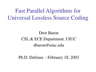
Fast Parallel Algorithms for Universal Lossless Source Coding
Explore the motivation, applications, and goals of lossless source coding, with a focus on parallel algorithms for efficient compression. Learn about source models, universality, semi-predictive methods, and achieving work-efficient algorithms for high compression quality. Discover the application of parallel compression to Bernoulli sequences and the benefits of fast, parallel coding.

Fast Parallel Algorithms for Universal Lossless Source Coding
E N D
Presentation Transcript
Fast Parallel Algorithms for Universal Lossless Source Coding Dror Baron CSL & ECE Department, UIUC dbaron@uiuc.edu Ph.D. Defense – February 18, 2003
Overview • Motivation, applications, and goals • Background: • Source models • Lossless source coding + universality • Semi-predictive methods • An O(N) semi-predictive universal encoder • Two-part codes • Rigorous analysis of their compression quality • Application to parallel compression of Bernoulli sequences • Parallel semi-predictive (PSP) coding • Achieving a work-efficient algorithm • Theoretical results • Summary
Motivation • Lossless compression: text files, facsimiles, software executables, medical, financial, etc. • What do we want in a compression algorithm? • Universality: adaptive to a large class of sources • Good compression quality • Speed: low computational complexity • Simple implementation • Low memory use • Sequential vs. offline
Why Parallel Compression ? • Some applications require high data rates: • Compressed pages in virtual memory • Remote archiving + fast communication links • Real-time compression in storage systems • Power reduction for interconnects on a circuit board • Serial compression is limited by the clock rate
Room for Improvement and Goals • Previous Art: • Serial universal source coding methods have reached the bounds on compression quality [Willems1998,Rissanen1999] • Parallel source coding algorithms have high complexity and/or poor compression quality • Naïve parallelization compresses poorly • Parallel dictionary compression [Franszek et. al.1996] • Parallel context tree weighting [Stassen&Tjalkens2001,Willems2000] • Research Goals: “good” parallel compression algorithm • Work-efficient: O(N/B) time with B computational units • Compression quality: as good as best serial methods (almost!)
Main Contributions • BWT-MDL (O(N) universal encoder): • An O(N) algorithm that achieves Rissanen’s redundancy bounds on best achievable compression • Combines efficient prefix tree construction with semi-predictive approach to universal coding • Fast Suffix Sorting (not in this talk): • Core algorithm is very simple (can be implemented in VLSI) • Worst-case complexity O(N log0.5(N)) • Competitive with other suffix sorting methods in practice • Two-Part Codes: • Rigorous analysis of their compression quality • Application to distributed/parallel compression • Optimal two-part codes • Parallel Compression Algorithm (not in this talk): • Work-efficient O(N/B) algorithm • Compression loss is roughly B log(N/B) bits
Source Models • Binary alphabet X={0,1}, sequence x XN • Bernoulli Model: • i.i.d. model • p(xi=1)= • Order-K Markov Model: • Previous K symbols called context • Context-dependent conditional probability for next symbol • More flexible than Bernoulli • Exponentially many states
P(xn+1=1|0)=0.8 0 leaf 0 01 11 P(xn+1=1|01)=0.4 1 0 internal node 1 P(xn+1=1|11)=0.9 Context Tree Sources root • More flexible than Bernoulli • More compact than Markov • Particularly good for text • Works for M-ary alphabet • State= context + conditional probabilities • Example: N=11, x=01011111111
Review of Lossless Source Coding • Stationary ergodic sources • Entropy rate H=limN H(x)/N • Asymptotically, H is the lowest attainable per-symbol rate • Arithmetic coding: • Probability assignment p(x) • Coding length l(x)=-log(p(x))+O(1) • Can achieve entropy + O(1) bits
Universal Source Coding • Source statistics are unknown • Need probability assignment p(x) • Need to estimate source model • Need to describe estimated source (explicitly or implicitly) • Redundancy: excess coding length above entropy (x)=l(x)-NH
Redundancy Bounds • Rissanen’s bound (K unknown parameters): E[(x)] > (K/2) [log(N)+O(1)] • Worst-case redundancy for Bernoulli sequences (K=1): (x*)=maxxXN {(x)} 0.5 log(N/2) • Asymptotically, (x)/N 0 • In practice, e.g., text, the number of parameters scales almost linearly with N • Low redundancy is still essential
S* Phase I Phase II y MDL Estimator x Encoder Semi-Predictive Approach • Semi-predictive methods describe x in two phases: • Phase I: find a “good” tree source structure S and describe it using codelength lS • Phase II: encode x using S with probability assignment pS(x) • Phase I: estimate minimum description length (MDL) tree source model S*=arg min {lS –log(pS(x))}
Arithmetic Encoder Determine s p(xi|s) s xi y S* Assign p(xi|s) Semi-Predictive Approach - Phase II • Sequential encoding of x given S* • Determine which state s of S* generated symbol xi • Assign xi a conditional probability p(xi|s) • Arithmetic encoding • p(xi|s) can be based on previously processed portion of x, quantized probability estimates, etc.
root node 0 node 11 node 01 unique sentinel Context Trees • We will provide an O(N) semi-predictive algorithm by estimating S* using context trees • Context trees arrange x in a tree • Each node corresponds to sequence of appended arc labels on path to root • Internal nodes correspond to repeating contexts in x • Leaves correspond to unique contexts • Sentinel symbol x0=$ makes sure symbols have different contexts
MDL structure for state s is or MDL structure for 1s additional structure 0s 1s 10s s s 00s Context Tree Pruning(“To prune or not to prune…”) • The MDL structure for state s yields the shortest description for symbols generated by s • When processing state s: • Estimate MDL structures for states 0s and 1s • Decide whether to keep 0s and 1s or prune them into state s • Base decision on coding lengths
1 1 1 1 0 0 0 0 Phase I with Atomic Context Trees • Atomic context tree: • Arc labels are atomic (single symbol) • Internal nodes are not necessarily branching • Has up to O(N2) nodes • The coding length minimization of Phase I processes each node of the context tree [Nohre94] • With atomic context trees, the worst-case complexity is at least O(N2) ☹
111 1 0 0 Compact Context Trees • Compact context tree: • Arc labels not necessarily atomic • Internal node are branching • O(N) nodes • Compact representation of the same tree • Depth-first traversal of compact context tree provides O(N) complexity • Theorem: Phase I of BWT-MDL requires O(N) operations performed with O(log(N)) bits of precision
Arithmetic Encoder Determine s p(xi|s) s xi y S* Assign p(xi|s) Phase II of BWT-MDL • We determine the generator state using a novel algorithm that is based on properties of the Burrows Wheeler transform (BWT) • Theorem: The BWT-MDL encoder requires O(N) operations performed with O(log(N)) bits of precision • Theorem:[Willems et. al. 2000]: redundancy w.r.t. any tree source S is at most |S|[0.5 log(N)+O(1)] bits
Assign p(xi(1)) Arithmetic Encoder 1 Arithmetic Encoder B Assign p(xi(B)) xi(1) p(xi(1)) x(1) y(1) Encoder 1 … … … x Splitter xi(B) p(xi(B)) x(B) y(B) Encoder B Distributed/Parallel Compression of Bernoulli Sequences • Splitter partitions x into B blocks x(1),…,x(B) • Encoder j{1,…,B} compresses x(j); it assigns probabilities p(xi(j)=1)= and p(xi(j)=0)=1- • The total probability assigned to x is identical to that in a serial compression system • This structure assumes that is known; our goal is to provide a universal parallel compression algorithm for Bernoulli sequences
Quantizer y k{1,…,K} rk ML(x) x Determine ML(x) Encoder Two-Part Codes • Two-part codes use a semi-predictive approach to describe Bernoulli sequences: • First part of code: • Determine the maximum likelihood (ML) parameter estimate ML(x)=n1/(n0+n1) • Quantize ML(x) to rk, one of K representation levels • Describe the bin index k with log(K) bits • Second part of code encodes x using rk • In distributed systems: • Sequential compressors require O(N) internal communications • Two-part codes need only communicate {n0(j),n1(j)}j{1,…,B} • Requires O(B log(K)) internal communications
r1 r2 rk rK bk bK b0 b1 b2 bk-1 Jeffreys Two-Part Code • Quantize ML(x) Bin edges bk=sin2(k/2K) Representation levels rk=sin2((2k-1)/4K) • Use K 1.772N0.5 bins • Source description: • log(K) bits for describing the bin index k • Need –n1 log(ML(x))-n0log(1-ML(x)) for encoding x
Redundancy of Jeffreys Code for Bernoulli Sequences • Redundancy: • log(K) bits for describing k • N D(ML(x)||rk) bits for encoding x using imprecise model • D(a||b) is Kullback Leibler divergence • In bin k, l(x)=-ML(x)log(rk )-[1-ML(x)] log(1-rk ) • l( ML (x)) is poly-line • Redundancy = log(K)+ l(ML(x))– N H(ML(x)) log(K) + L • Use quantizers that have small L distance between the entropy function and the induced poly-line fit
Redundancy Properties • For xs.t. ML(x) is quantized to rk, the worst-case redundancy is log(K)+N max{D(bk||rk),D(bk-1||rk)} • D(bk||rk) and D(bk-1||rk) • Largest in initial or end bins • Similar in the middle bins • Difference reduced over wider range of k for largerN (larger K) • Can construct a near-optimal quantizer by modifying the initial and end bins of the Jeffreys quantizer
Redundancy Results • Theorem: The worst-case redundancy of the Jeffreys code is 1.221+O(1/N) bits above Rissanen’s bound • Theorem: The worst-case redundancy of the optimal two-part code is 1.047+O(1) bits above Rissanen’s bound
x(1) y(1) n0(1),n1(1) ML(x) rk x(1) … ML(x) [jn0(j)] / [j n0(j)+j n1(j)] Quantizer … n0(B),n1(B) y(B) x(B) k x(B) Encoder 1 Encoder B Determine n0(B) and n1(B) Determine n0(1) and n1(1) Parallel Universal Compression for Bernoulli Sequences • Phase I: • Parallel units (PUs) compute symbol counts for the B blocks • Coordinating unit (CU) computes and quantizes the MDL parameter estimate ML(x) and describes k • Phase II: B PUs encode the B blocks based on rk
x(1) y(1) x … … … Splitter Compressor 1 x(B) y(B) Compressor B Why do we need Parallel Semi-Predictive Coding? • Naïve parallelization: • Partition x into B blocks • Compress blocks independently • The redundancy for a length-N/B block is O(log(N/B)) • Total redundancy is O(B log(N/B)) • Rissanen’s bound is O(log(N)) • The redundancy with naïve parallelization is excessive!
x(1) y(1) x(1) symbol counts 1 S* … … symbol counts B y(B) x(B) Phase I Phase II x(B) S* Compressor 1 Compressor B Coordinating Unit Statistics Accumulator B Statistics Accumulator 1 Parallel Semi-Predictive (PSP) Concept • Phase I: • Bparallel units (PUs) accumulate statistics (symbol counts) on the B blocks • Coordinating unit (CU) computes the MDL tree source estimate S* • Phase II:-- B PUs compress the B blocks based on S*
Describe S* structure Coordinating Unit Describe bin indices {ks}sS* S* {ks}sS* Determine p(xi(b)|s) s p(xi(b)|s) Arithmetic Encoder xi(b) Determine s y(b) Parallel unit b p(xi(b)|s)1{xi(b)=1}rks+1{xi(b)=0}(1-rks ) Source Description in PSP • Phase I: the CU describes the structure of S* and the quantized ML parameter estimates {ks}sS* • Phase II: each of B PUs compresses block x(b) just like Phase II of the (serial) semi-predictive approach
Dmax 2Dmax=O(N/B) Complexity of Phase I • Phase I processes each node of the context tree [Nohre94] • The CU processes the states of a full atomic context tree of depth-Dmax, where Dmax log(N/B) • Processing a node: • Internal node: requires • O(1) time • Leaf: CU adds up block • symbol counts to compute • each symbol count, i.e., ns=b ns(b), where {0,1} • The CU processes a leaf node in O(B) time • With O(N/B) leaves, the aggregate complexity is O(N), which is excessive
Phase I in O(N/B) Time • We want to compute ns=b ns(b) faster • An adder tree incurs O(log(B)) delay for adding up B block symbol counts • Pipelining enables us to generate a result every O(1) time • O(N/B) nodes, each requiring O(1) time
Parallel unit b Determine p(xi(b)|s) s p(xi(b)|s) Arithmetic Encoder xi(b) Determine s y(b) S* {ks}sS* Phase II in O(N/B) Time • The challenging part in Phase II is determining s: • Define the context index for a length-Dmax context s preceding xi(b) as the binary number that represents s • The length-2Dmaxgenerator table g satisfies gj=sS* if s is a suffix of the context whose context index is j • We can construct g in O(N/B) time (far from trivial!) • Compute context indices for all symbols of x(b) and determine the generating states via the generator table g
S*,{ks}sS* Decoding Unit 1 Decoding Unit B x(1) DEMUX y(1) Reconstruct S*,{ks}sS* … … … bus y x(B) y(B) Decoder • An input bus is demultiplexed to multiple units • The MDL source and quantized ML parameters are reconstructed • The B compressed blocks y(B) are decompressed on B decoding units
Theoretical Results • Theorem: With computations performed with 2 log(N) bits of precision defined as O(1) time: • Phase I of PSP approximates the MDL coding length within O(1) of the true optimum • The PSP algorithm requires O(N/B) time • Theorem: The PSP algorithm uses a total of O(N) words of memory = a total of O(N log(N)) bits • Theorem: The pointwise redundancy of PSP w.r.t. S* is (x) < B[log(N/B)+O(1)]+|S|*[log(N)/2+O(1)] parallelization overhead
Main Contributions • BWT-MDL (O(N) universal encoder): • An O(N) algorithm that achieves Rissanen’s redundancy bounds on best achievable compression • Combines efficient prefix tree construction with semi-predictive approach to universal coding • Fast Suffix Sorting (not in this talk): • Core algorithm is very simple (can be implemented in VLSI) • Worst-case complexity O(N log0.5(N)) • Competitive with other suffix sorting methods in practice • Two-Part Codes: • Rigorous analysis of their compression quality • Application to distributed/parallel compression • Optimal two-part codes • Parallel Compression Algorithm (not in this talk): • Work-efficient O(N/B) algorithm • Compression loss is roughly B log(N/B) bits
More… • Results have been extended to |X|-ary alphabet • Future research can concentrate on: • Processing broader classes of tree sources • Problems in statistical inference • Universal classification • Channel decoding • Prediction • Characterize the design space for parallel compression algorithms
Generic Phase I • if (s is a leaf) { • Count symbol appearances ns0 and ns1 • MDLslength(ns0, ns1) • } else { /* s is an internal node */ • Recursively compute MDL length and counts for 0s and 1s • ns0 n0s0+n1s0, ns1 n0s1+n1s1 • MDLslength(ns0, ns1) • if (MDLs >MDL0s +MDL1s ) • Keep 0s and 1s • } else { • Prune0s and 1s, keeps • } • }