Download
1 / 15
150 likes | 354 Vues
The Environmental Cost Curve. An economic approach to the environment production trade-off Jack Sinden Agricultural and Resource Economics School of Economics University of New England Armidale NSW. 1 Introduction: the ideal & the difficulty.

E N D
The Environmental Cost Curve An economic approach to the environment production trade-off Jack Sinden Agricultural and Resource Economics School of Economics University of New England Armidale NSW
1 Introduction: the ideal & the difficulty • Economists try to value all benefits and costs • So the ideal trade-off is the monetary value of the environmental gain against the monetary value of the associated production loss. • But,usually we cannot value environmental benefits in monetary terms.
1 Introduction: a partial solution Whereas, usually we can estimate production losses at different levels of environmental gain The measurable trade-off is therefore the monetary value of lost production against increasing levels of environmental outcome The graph of losses/outcomes may be called the the environmental cost curve
1 Introduction: objectives • To illustrate the nature and derivation of the environmental cost curve, and • To discuss the interpretation and role of the cost information • (These are the economist’s marginal cost curves)
1 Introduction: context • Economists can provide information: • Costs, their distribution, which kind of farm bear highest (lowest) costs Australian Forestry 2005 • Do the benefits exceed the costs ? • The Rangeland Journal 2004 • Economists can give their own professional views: • Farm Policy Journal 2005
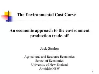
2 Nature of environmental cost curves They are the economist’s marginal cost curves. So we produce goods in order of increasing cost, and define cost as the cost of the last unit produced. So if we protect all vegetation on 50 farms, marginal cost is the highest cost per ha over all 50 farms. If we protect X%of the vegetation, we identify the least-cost X%, and marginal cost is the highest cost per ha over that X%.
2 Nature of environmental cost curves Linear Cost $ per ha 70 50 1 Curvi-linear 20 2 100% 0 70% Environmental gain: area of native vegetation protected
3 Measurement of production cost • We can measure production cost in three ways: • Gross margin per ha=Money revenues - money costs • Farm business profit= Gross margin - fixed costs- depreciation - return to capital - owners salary • Return to land = (GM - fixed costs- depreciation - salary)/price paid for land, as a %
3 Measurement of production cost • Production cost is the loss in any one of these three measures of income to obtain the environm’tal gain • measured in actual units (GM in $, FBP in $, or RETL in %), and • expressed as % loss of existing income, or % loss of potential income
4 Measurement of environmental gain • Potential measures of environmental gain • Decreases in level of salinity • Increases in environmental flows of water • Actual applications in environmental cost curves • Emissions of greenhouse gas - decreases • Emission of pollutants that => acid rain - decreases • Area of native vegetation protected - increases
5 An application to vegetation protection • Location: Moree Plains Shire: Sinden 2005 FPJ • Objectives: to determine trends in loss of gross margin • Data: from face to face survey of 51 farms. • Cost is loss in GM, as % of existing farm income. • So a 96.9% loss means loss is +- equal to existing GM, & so existing GM could be +- doubled if…
5 An application to vegetation protection The cost curve Cumulative area protected Highest % loss GM 10 2.0* 20 2.1 97 80.5 100 96.9 * If 10% of the area is protected, the highest loss amongst all farms involved is 2.0 % of existing income
6 Discussion • Provides information for the problem at hand: • Some vegetation can be protected at a very low cost • Some vegetation can be protected only at a very high loss of income • Is this latter high cost justified for protection of this particular vegetation?
6 Discussion • Provides information for a more general interpretation: • These trends are likely to be general for all regions and all kinds of vegetation • So the major question for the community seems to be: • How much native vegetation should we protect?