Download
1 / 35
360 likes | 503 Vues
On the Complexity of Join Predicates. Jeff Naughton with Jin-Yi Cai, Venkatesan Chakaravarthy,Raghav Kaushik, Jignesh Patel, Karthikeyan Ramasamy. Outline. What are joins and join predicates? What issues arise with respect to joins in the presence of new data types?

E N D
On the Complexity of Join Predicates Jeff Naughton with Jin-Yi Cai, Venkatesan Chakaravarthy,Raghav Kaushik, Jignesh Patel, Karthikeyan Ramasamy
Outline • What are joins and join predicates? • What issues arise with respect to joins in the presence of new data types? • Theoretical discussion of “difficulty” of join predicates.
Join: Useful Combination • R join_{pred} S is defined to be: • form cross product of R and S • apply selection (using pred) to the result • The “workhorse” operator of relational systems, used in every non-trivial query.
Example of a Join • Suppose we have two tables: • Students(sid, name, …) • Grades(courseId, sid, grade) • and we want a list of student names and grades, then we do: • Students join_{sid=sid} Grades • This is an equijoin, since pred is =.
In SQL... SELECT * FROM Students, Grades WHERE Students.sid = Grades.sid
Grades cid sid grade 245 1 A 245 2 C 311 1 A Students sid name 1 Garcia 2 Naughton Result sid name cid grade 1 Garcia 245 A 2 Naughton 235 C 1 Garcia 345 A Example
How should we evaluate joins? • 200+ citations in DBLP bibliography • Most obvious (and slow!) algorithm: nested loops join. for each tuple r in R for each tuple s in S if join-pred(r,s) then output (r,s)
In the beginning... • Goal was: find a better algorithm than nested loops for equijoins. • Two early contenders [BE77]: • sort-merge join • index nested-loops join • Both much better than nested loops, but not as good as partition-based joins.
R1 S1 S1 R1 S2 R2 S R S3 R3 S2 R2 S4 R4 vs. vs. Intuition behind partition joins
New Topic: Adding Types to DBMS • What types do Relational DBMS handle? • Tables, Rows, Attributes • Attributes drawn from very restricted domains: essentially • numeric • string
Object/Relational DBMS • A lot of hype a few years ago, marketing lingo was “universal server.” • Beyond the hype, all major relational systems are incorporating some O/R features. • What does O/R add? Of interest today: • new domains (types) • set-valued attributes
Some examples... • Spatial attributes • landUse(id: integer, outline: polygon); • county(name: string, boundary: polygon); • Set-valued attributes • students(id:int, coursesTaken: set of courseId); • courses(id: courseId, preReqs: set of courseId);
What does this have to do with joins? • The following is a “join” query: • For each county, list the types of land use that exist within the county. • Here the “join predicate” is polygon overlap. In extended SQL, we have: Select * From county, landUse Where county.boundary overlaps landUse.outline
Another example: • For each student, list the courses she is eligible to take. • Here, the join predicate is set containment: Select * From student, course Where course.preReqs subsetof student.coursesTaken.
Learning from equijions.. • The best general equijoin algorithms work by partitioning input relations. • Can we find good partitioning-based algorithms for spatial joins and set containment joins?
Spatial Joins… • DBLP bibliography lists 50 references for spatial join algorithms. • Best in absence of index is some flavor of partition-based join. • Not as clean as equijoin algorithms. • Involve replication of data and/or duplication of computation. • Seems to be tougher than equijoins.
Set-Containment Joins • Much less work to date. • Two main approaches: • signature nested loops [HM96,HM97] • partition-based algorithms [HM97, RPNK00] • Signature-based approach: nested loops, but reduces the cost of the comparisons. • Partition based - complex, huge design space.
C1 S1 S2 C2 Replication vs. Extra Joins Courses(245, {1, 4}) Students(23, {1, 4, 5}) Courses(311, {4,5}) Students(23, {1, 4, 5}) Then we have avoided joining (C2, S1), but at the expense of replicating Students(23, {1, 3, 5}). Then we need to join (C1, S1) and (C2, S1).
Can we prove that joins over these domains are hard? • Big problem: everything is in P • in fact, in quadratic time. • How can we distinguish between them? Our initial progress: • combinatorial complexity • difficulty of finding “optimal” algorithm.
Abstracting Join Algorithms • Represent join by a bipartite graph. • One node per tuple of R • One node per tuple of S • an edge from node r to node s if the tuple r joins with the tuple s.
Pebbling Game • Represent computation by a pebbling game • two pebbles, one for R, one for S • place tuples on both ends of an edge, remove it • goal: remove all edges.
The pebbling game: R (join) S
Our use of the pebble game • To attempt to capture relative difficulty of different join problems. • Intuition: at some point any join algorithm must consider each edge of the join graph. • That moment is captured by placing pebbles on that edge. • Length of pebbling sequence an indication of how efficiently these moments can be ordered.
Metric: # pebble moves. • (G) (required pebble moves) (#connected components in G) • Intuition: • any pebbling scheme must pay “startup cost” of one pebble move per component. • Want to factor this out.
Easy bounds on (G) • Theorem: for a graph with m edges, m - 1 (G) < 2m • Why? • at best, each pebble move removes an edge; • at worst, each pair of pebble moves remove an edge.
Tighter bound on (G) • Theorem: for a connected m edge graph, we have that (G) 1.25m 1. • Proof idea: find a partition of the edge set E1, E2, …, Ek, where • at most one of the Ei has |Ei| <= 4. • each of the Ei can be pebbled in |Ei| moves. • Uses DFS tree embedded in graph and repeatedly eliminates components “at the fringe.”
Lower bound on worst case • Theorem: there is a family of graphs for which (G) = 1.25m. G3 G4 G5
Status check... • Worst case join graphs require about 1.25m • Best case join graphs can be pebbled in m. • Not much “wiggle room” between the two.
Equijoins • Equijoin: can show (G) = m. • Why? For equijoins, join graph is a union of complete components. • So, by this metric, no join predicate is easier than equality.
Spatial and Set-Containment Joins • Can show that (G) can reach 1.25m. • So by this metric no join is harder than these joins. • Proof idea: show that these join predicates are “universal”: • for any bipartite graph G, there is an instance of a {set, overlap} join J such that G is the join graph for J
Next Topic: Finding Pebblings • Recall that for equijoins, (G) = m. • So, given an arbitrary equijion graph, how hard is it to find a pebbling sequence of cost m? • Answer: Can do this in linear time.
What about set containment joins and spatial overlap joins? • Recall that for these joins, (G) can range from m to 1.25m. • Can you find the best pebbling efficiently? Unlikely! • Theorem: for set containment joins and spatial overlap joins, finding optimal pebbling sequence is NP-Complete. (Follows from [MKY81,NW97].)
So how about approximating? • Theorem: for any join graph of m edges, can find a pebbling of cost 1.25m in linear time. • Raises question: can you find a polynomial time approximation scheme?
Answer appears to be “no” • Theorem: The pebbling problem for set containment and spatial overlap joins is MAX-SNP-Complete. • Proof idea: • Has a constant factor approx. algorithm (so in MAX-SNP). • MAX-SNP-Complete by L-reduction from TSP-3(1,2), which in turn is MAX-SNP-Complete by reduction from TSP-4(1,2).
Conclusion: In this model... • equality easiest join predicate • can be pebbled in m moves • pebbling can be found in linear time • polygon overlap, set containment hardest. • Exist instances that take 1.25m moves • Finding pebbling is NP-complete and MAX-SNP-Complete