Download
1 / 17
170 likes | 303 Vues
This document presents a novel methodology for beach management via ensemble modelling, aimed at diagnosing and predicting beach retreat due to varying sea level rise scenarios. Utilizing numerical models such as Leont’yev, SBEACH, as well as static models like Edelman, Bruun, and Dean, the tool assesses beach retreat under diverse conditions. The effectiveness of this ensemble approach exceeds traditional tools, providing reliable predictions with minimal field data. This tool has been validated through extensive experimentation and offers significant benefits for coastal management locally and globally.

E N D
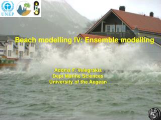
Beach modelling IV: Ensemble modelling Adonis F. Velegrakis Dept Marine Sciences University of the Aegean
Synopsis • Why model ensembles • Method • Effectiveness and benefits 4 Tool explained
1 Why model ensembles Development of a new methodology/tool for beach management which may diagnose/predict beach retreat: • Under different long-term and short-term sea level rise • And for different morphological, hydrodynamic and sedimentological conditions And which can be used locally and globally and will be better than existing tools
2 Method • Beach retreat is assessed through the numerical models Leont’yev και SBEACHand the static models Edelman, Bruun and Dean. • These models have been already run for linear profiles as well as non-linear (natural) profiles and for many environmental conditions • The models can be run individually, or better use them as ensembles (Rixen et al., 2007) as: • (i)Leont’yev, SBEACH, Edelman: ‘short-term’ (storm surges) • (ii)Bruun and Dean‘long-term’ ASLR)
2 Method (cont.) The models have been run for different conditions (> 19000 experiments) (results are stored in the data base estimator): • beach slope (1/10, 1/15, 1/20, 1/25, 1/30), • wave conditions (Η=1, 1.5, 2, 2.5, 3, 4, 5, 6 m και T= 3 - 14 s) • sediment size (d50=0.2, 0.33, 0.50, 0.80, 1, 2 και 5 mm) For 14scenaria of sea level rise (0.038, 0.05, 0.10, 0.15, 0.22, 0.30, 0.40, 0.50, 0.75, 1, 1.25, 1.5, 2 και 3 m). The model ensembles have been also used for natural profiles from DUCK, n. Carolina and Christchurch Bay, UK (> 3000 experiments). The results from natural and linear profiles have been compared. Moreover, the results have been compared with those by a Boussinesq model (> 1100 experiments)
3 Effectiveness and benefits The tool has been shown to be quite effective when was compared with results from the state-of-the-art Boussinesq model , which has been validated by physical experiments The major advantage of the present tool is that requires minimum field information for an initial assessment. If however such information is available then the range of the prediction envelope can be reduced The tool consists of 3 platforms [1] Coastal retreat estimator on the basis of an existing data base; [2] Coastal retreat estimator- static models; and [3] Coastal retreat estimator-dynamic models
Beach retreat under storm surges • Lower limit: • s= 0.54α2+7.08α - 0.31 • (R2 = 0.99) • Higher limit: • s= 1.23α2+29.52α+4.71 • (R2 = 0.99) • Where s beach retreat (in m) and αsea level rise (in m). Fig. 1 Estimations of beach retreat (16384 experiments) by the models Leont’yev, SBEACH και Edelman. x-axis, sea level rise; y-axis beach retreat
Long-term beach retreat • Lower limit • s= -0.001α2+7.9α + 0.1 • (R2 = 0.99) • Higher limit: • s= 5Ε-05α2+28α+5.2 • (R2 = 0.99) • Where s beach retreat (in m) and αsea level rise (in m). Fig. 2 Estimations of beach retreat usingthe models Bruun and Dean (2752 experiments). x-axis, sea level rise; y-axis beach retreat; yellow dash line, mean limits
Beach retreat under storm surges Natural profiles- Results not stored in the data base estimator Fig. 3.Result ranges from models of the short-term ensemble for natural profile (mean profile from Delilah experiment in DUCK). x-axis, sea level rise; y-axis beach retreat; black dash line, mean limits
Comparison between linear (γραμμικές) and natural profiles Leont’ yev SBEACH Edelman ~16% maximum deviation 30% maximum deviation ~10% maximum deviation Fig. 4.Comparisons of the results from 3 models (short-term ensemble) between linear (blue lines) and natural profiles- SandyDuck experiment (red lines) x-axis, sea level rise; y-axis beach retreat. 1 Bed slopes in natural and linear profiles have been compared at the swash zones
Comparison between linear (γραμμικές) and natural profiles for the long-term ensemble Bruun Dean 6.7% maximum deviation1 6.3% maximum deviation Fig. 5.Comparisons of the results from 3 models (long-term ensemble) between linear (blue lines) and natural profiles- SandyDuck experiment (red lines) x-axis, sea level rise; y-axis beach retreat. 1 Bed slopes in natural and linear profiles have been compared at the active profile (Bruun) and the surf zone (Dean)
The unified ensemble shows similar range with the Boussinesq model 6.3% maximum deviation Mean limits of the unified ensemble Lower limit: s= 0.33 α2 + 7.4 α – 0.14(R2 =0.99) Higher limit : s= 0.74 α2 + 28.9 α + 4.9(R2 =0.99) Fig. 6.The mean limits of the predictions of the unified ensemble 2 together with comparisons of the predictions of the short- and long-term ensembles and the unified ensemble with the Boussinesq model predictions.
slope 1/20 H = 1.20 m, T = 5s, d50 = 0.3 mm Slope 1/10 Slope 1/15 Fig. 7. Comparison of Boussinesq results with the experiments of Dette et al. (1998) (HYDRALAB). Blue line, initial profle; red line final profile; dots experimental data. (Monioudi, 2011).