Download
1 / 16
420 likes | 1.21k Vues
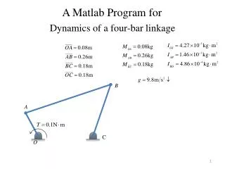
A Matlab Program for. Dynamics of a four-bar linkage. B. A. C. O. Mass matrix and external force vector . Jacobian matrix and γ. Computation. A convenient way with Matlab solver . Solve initial value problems for ordinary differential equations with ode45(commended), ode23, ode113…

E N D
A Matlab Program for Dynamics of a four-bar linkage B A C O
A convenient way with Matlab solver Solve initial value problems for ordinary differential equations with ode45(commended), ode23, ode113… The equations are described in the form of z‘=f(t,z)
The syntax for calling solver in Matlab A vector of initial conditions Solution array [T,Z] = ode45(@Func4Bar,[0:0.005:2],Z0); column vector of time points A vector specifying the interval of integration A function that evaluates the right side of the differential equations functiondz=Func4Bar(t,z) global L1 L2 L3 L4 torque gravity phi1=z(3); phi2=z(6); phi3=z(9); dphi1=z(12); dphi2=z(15); dphi3=z(18); M=diag([L1 L1 L1^3/12 L2 L2 L2^3/12 L3 L3 L3^3/12]); J=[ -1 0 -0.5*L1*sin(phi1) 0 0 0 0 0 0; 0 -1 0.5*L1*cos(phi1) 0 0 0 0 0 0; 1 0 -0.5*L1*sin(phi1) -1 0 -0.5*L2*sin(phi2) 0 0 0; 0 1 0.5*L1*cos(phi1) 0 -1 0.5*L2*cos(phi2) 0 0 0; 0 0 0 1 0 -0.5*L2*sin(phi2) -1 0 -0.5*L3*sin(phi3); 0 0 0 0 1 0.5*L2*cos(phi2) 0 -1 0.5*L3*cos(phi3); 0 0 0 0 0 0 1 0 -0.5*L3*sin(phi3); 0 0 0 0 0 0 0 1 0.5*L3*cos(phi3)];
The syntax for calling solver in Matlab J=[ -1 0 -0.5*L1*sin(phi1) 0 0 0 0 0 0; 0 -1 0.5*L1*cos(phi1) 0 0 0 0 0 0; 1 0 -0.5*L1*sin(phi1) -1 0 -0.5*L2*sin(phi2) 0 0 0; 0 1 0.5*L1*cos(phi1) 0 -1 0.5*L2*cos(phi2) 0 0 0; 0 0 0 1 0 -0.5*L2*sin(phi2) -1 0 -0.5*L3*sin(phi3); 0 0 0 0 1 0.5*L2*cos(phi2) 0 -1 0.5*L3*cos(phi3); 0 0 0 0 0 0 1 0 -0.5*L3*sin(phi3); 0 0 0 0 0 0 0 1 0.5*L3*cos(phi3)]; gamma=[ 0.5*L1*cos(phi1)*dphi1^2; 0.5*L1*sin(phi1)*dphi1^2; 0.5*L1*cos(phi1)*dphi1^2+0.5*L2*cos(phi2)*dphi2^2; 0.5*L1*sin(phi1)*dphi1^2+0.5*L2*sin(phi2)*dphi2^2; 0.5*L2*cos(phi2)*dphi2^2+0.5*L3*cos(phi3)*dphi3^2; 0.5*L2*sin(phi2)*dphi2^2+0.5*L3*sin(phi3)*dphi3^2; 0.5*L3*cos(phi3)*dphi3^2; 0.5*L3*sin(phi3)*dphi3^2]; g=[0 gravity*L1 torque 0 gravity*L2 0 0 gravity*L3 0]'; Matrix=[M J'; J zeros(size(J,1),size(J,1))]; d2q=Matrix\[g;gamma]; dz=[z(10:18,:); d2q(1:9,:)];
A slider-crank mechanism B C A O G